1.    INTRODUCTION

1.1  Problem Statement

A Coronal Mass Ejection (CME) is a significant eruption of plasma and tangled magnetic fields from the Sun’s Corona out into the Heliosphere. During Solar Maxima, the Sun can produce several CMEs each month, a small percentage of which traverse interplanetary space and are directed toward Earth. When they collide with the Earth’s Magnetosphere, it triggers severe geo-magnetic storms. These storms have the potential to disrupt satellite communication, corrupt satellite data, and induce currents that reach the Earth’s atmosphere and damages infrastructure, both ground-based, and Low Earth Orbit (LEO)- based. Historical Events such as the Carrington event is an example of the potential damage and years of affect that CMEs can cause. As modern society becomes increasingly reliant on satellite-based systems, and as space missions venture closer to the Sun, even routine CMEs can pose growing risks. However, accurately identifying reliable patterns and early precursors of CME behaviour remains a major gap in our space weather understanding and prediction. This uncertainty highlights a growing need for improved analysis and cross-validation of solar observation data.

1.2 Significance and Impact

A Coronal Mass Ejection (CME) is a massive expulsion of plasma and intertwined magnetic fields. CMEs originate from the Sun's corona, and when they make it through the heliosphere, they are known as interplanetary CMEs or ICMEs. Some of the ICMEs propagate towards Earth, and when they interact with our magnetic field, they trigger geomagnetic storms, disrupt satellite communications, and have the potential to even disrupt ground-based infrastructure and technology systems.   The real-world consequences of CMEs are undeniably large. For a succinct example, during the unveiling of the Starlink satellites in February 2022, a CME hit Earth, and introduced dense gases into LEO (Low Earth Orbit), which caused immense drag on the satellites, destroying over 38 out of the 49 planned satellites of the Starlink mission. Consequently, this event silently cost SpaceX approximately $50 million. This incident is just one of many that displayed the true destructive power of even moderate ICMEs.

Historically, the most severe example of CME interaction with humanity was the Carrington Event of 1859. During this event, intense geomagnetic storms shook the Earth, with aurorae observable throughout the globe. Additionally, telegraph stations were deemed useless, and wires sparked due to the intense CMEs that the Earth was exposed to. In the rare scenario that such an event was to happen today, it would induce a noticeably greater impact due to the ever-increasing dependence we have on technology.   As modern society’s technological reliance grows ever deeper, CMEs pose an increasingly greater risk. Even though this risk is growing ever more, it is hardly talked about as a mere threat to our technological reliance. Thus, it is significant to hunt for patterns in CME and sunspot data to reliably predict periods of increased space weather risk, and to mitigate the effects of CMEs.   To address these challenges, this project investigates whether multi-mission solar observations can reveal reliable patterns associated with CMEs.

3.     Methodology

3.1 Main Methodology Structure

This project employs an observational and analytical methodology to investigate the destructive potential of Coronal Mass Ejections (CMEs), using Heliospheric and spacecraft to investigate relationships between sunspot characteristics, CME abundance and morphology and the solar cyclic activity to predict periods of increased risk.

The structure follows a sequential data process resulting in the isolation of significant risk solar events which usually consist of periods of increased magnetic helicity, CME propagation, sunspot complexity, and thus a higher likelihood of Earth-impact. These events are traced from their original regions on the solar surface and their original timestamp during the solar cycle of the Sun.

Since no single spacecraft can observe the entire surface of the Sun and propagation of Earth directed CMEs, this project scours through information from spacecraft based on different points in the Sun’s orbit, helping in the cross-validation of data and to provide a basis for temporal and spatial analysis. Coronal Imaging instruments can help us to understand the visible characteristics and morphology of the solar surface, in-situ measurements provide a basis for understanding the deep morphology and the production characteristics of the ejecta, and together these systems could help resonate visible solar processes to the internal morphology of ejecta. This multi-mission approach enables cross-validation and minimizes observational bias.

Using these selected datasets, graphical analysis is performed to compare temporal evolution, speed profiles, and geomagnetic response indicators. Only events meeting predefined impact or intensity thresholds are included to maintain methodological consistency. Mathematical analysis is then used to identify recurring patterns and relationships between sunspot and Earth direct CMEs, and the outcome will result in a dataset suitable for identifying patterns between sunspot classification, CME propagation, morphology of solar ejecta and geomagnetic saliency.

3.2 Data Collection

The data that will be used for this project will be systematically collected from a large basis of space-based observatories and solar monitoring missions to study coronal mass ejections, sunspots, and their resonance with solar flares. The data timestamps and temporal analysis will be focused on periods of intense CME risk by analysing the Solar Cycles 22, 23, 24 and 25 (which is our current solar cycle). This wide range of data from 4 solar cycles will provide information to identify precursors, patterns, and potential risks to Earth and space-based technologies without including periods of Maunder Minimum that will skew models and data predictions.

The primary sources of data will include SOHO ( Solar and Heliospheric Observatory) and SDO (Solar Dynamics Observatory) for detailed imaging of sunspots, solar flares, and CME morphology; DSCOVR, ACE, and Aditya L1 for in-situ measurements of solar wind, plasma density, and magnetic field orientation; STEREO-A for multi-angle observations of CME propagation; and IRIS, Parker Solar Probe, and Solar Orbiter for high-resolution observations of the solar corona and chromosphere. Together, these missions will provide complementary datasets to ensure both global coverage and precise measurements of solar phenomena from all physical angles to prevent a rudimentary basis of developmental understanding.

For each event and period taken into account, the propagation period, speed, width, trajectory, Bz component, sunspot group of origin, sunspot classification (α, β, γ, δ), and flare class (C, M, X) will be recorded. These measurements will allow for a systematic and fair comparison of events and determine repeating precursors for solar events of different significance.

To ensure a robust understanding, particularly about Earth-directed CMEs, the data will follow a strict criteria where only events with reliable multi-mission observations will be included. On the other hand, CMEs with limited data and incomplete trajectory information will be excluded. This selection criteria will ensure the dataset emphasizes occurrences with the highest priority and threat to space-based communication systems.

Through this structured methodology, the project will establish a robust dataset capable of supporting pattern recognition, CME classification, and prediction of periods of increased risk in solar activity.

3.3 Cross-Validation Approach

During the process of data selection, all data chosen and collected will be ensured to follow utmost quality and be limited on bias and skewed numbers. To cross-check and to ensure the validity of data, all datasets collected will be cross-validated by multiple solar observatories operating during different timestamps and at different angles of the sun, providing a larger spectrum of solar phenomena.

For a succinct example, CME activity observed by SDO or SOHO will be cross-validated by STEREO-A using a Multi-spacecraft triangulation. This method will be employed to round off chances of significant projection & instrumental bias. Instrumental uncertainties and observational limitations, such as data gaps or reduced temporal resolution, will be documented for each event to maintain transparency and reliability.

This method of cross-validation will help to develop a more robust and multi-faceted understanding of CMEs and their processes.

3.4 Limitations

Even within the project’s strict criteria for choosing events and solar phenomena with minimal bias and multi-angular observation to cross-validate using triangulation, bias and false data may still be an issue. These issues are constrained, however, instrument bias may skew data and similar prediction models. In turn, this false data can cause limitations in the real-world applications of identifying CME data.

Additionally, temporal resolution differences between instruments may introduce inconsistencies when determining CME onset time, peak acceleration, or propagation speed. Even when events are observed across multiple spacecraft, variations in imaging cadence and processing algorithms may result in small but significant deviations in measured parameters. These discrepancies may influence derived indices or classifications developed within this study.

Another limitation arises from assumptions made during three-dimensional reconstruction and triangulation. CME structures are highly dynamic and may not conform to simplified geometric models, which can introduce uncertainties when estimating trajectory, or expansion rates. As a result, some reconstructions may represent approximations rather than exact physical values.

Environmental factors within the heliosphere, such as solar drag, background magnetic field variability, and interactions with preceding CMEs, may also alter CME propagation after launch. Because these external influences are not always fully captured within observational datasets or predictive models, the resulting analysis may not account for all dynamic processes affecting CME evolution.

Finally, while efforts are made to minimize bias through strict selection criteria and cross-validation, the availability of high-quality multi-spacecraft data limits the total number of usable events. This constraint may reduce available data, meaning that conclusions provided by this dataset should be interpreted as indicative trends rather than fully mature rules governing all CME behavior.

2.    Background Research

2.1 Causes of CMEs and Sunspots

2.1.1 Causes of CMEs

Coronal Mass Ejections (CMEs) are massive expulsions of bubbles of plasma released through the Sun’s corona (outer layer of the sun), and they propagate towards interplanetary space. The rope-like part of a CME is known as flux ropes. These flux ropes are made of plasma and magnetic field lines. Additionally, they originate close to the Lower Corona and make their way over Polarity Inversion Lines (PILs). PILs are a critical boundary near the Sun’s corona, where the stored energy inside a magnetic field (non-potential) turns into eruptive magnetic structures. CMEs can only be initiated when the magnetic field is not in a potential state and is instead in a state of free magnetic energy (the excess energy in the corona overcoming the potential state). In magnetohydrodynamics, potential magnetic energy is denoted by V x B= 0 where V is plasma velocity and B is magnetic field and the formula shows the interaction between the two. This is because under the potential state there is no magnetic current. Consequently, this zone is one of the most active zones and propagates in the creation of flux ropes.

Coronal Mass Ejections are generally caused by stressed, strong, and twisted flux ropes that are highly unstable, snapping and then reconnecting with sheer force, propelling plasma out of the lower corona. When these flux ropes with magnetic helicity transfer their magnetic complexity from the photosphere to the corona, it creates a magnetic field parallel to the horizontal surface of the sun caused by the solar convection currents dragging on the surface. When this horizontal plasma flows on the surface, it introduces shearing and twisting motions, injecting magnetic helicity and energy from the solar interior to interplanetary space. The corona cannot break magnetic helicity due to its high electrical conductivity hence it makes the corona to remain in a state of ideal magnetohydrodynamics and preserving the helicity of magnetic flux ropes. Furthermore, CMEs are efficient breakers of helicity, hence after a period of intense CME activity, the corona loses most of its helicity, pushing the Sun into a period of inactivty. There are myriads of different types of coronal mass ejections: Here is a succinct list. ·        ICMEs—Interplanetary CMEs, or ICMEs, are CMEs that propagate out of the lower corona and make their way into space. These ICMEs are quite powerful compared to CMEs that are local within the heliosphere of the sun. ·        Halo CMEs—These CMEs are CMEs that are directed towards Earth and have the potential to cause geomagnetic storms and significant satellite and radio technology-based disruptions. ·        Slow CMEs—These CMEs are under 400 km/s and thus take longer to reach Earth. Consequently, they cause little to no intense geomagnetic effects on Earth. ·        Fast CMEs—These CMEs are over 800 km/s, and thus reach Earth faster with more momentum. Consequently, they generate strong geomagnetic storms and hail from more active regions of the sun during solar maxima. ·        Coronal Hole Stream CMEs—These CMEs originate from coronal holes, which are regions with open magnetic field lines that tend to launch slower and long-lasting streams of plasma. These CMEs are associated with high-speed streams, in turn causing recurring geomagnetic activity. ·        Magnetic-Cloud CMEs—These CMEs have a defined magnetic structure and are made up of twisting flux ropes that cause a greater geomagnetic impact. Magnetic-cloud CMEs are a type of ICME that reach interplanetary space. ·        Narrow CMEs—These CMEs have a small angular width when observed while ejected from the sun. The qualifying angular width is about 10 degrees when propagating out of the heliosphere. In comparison, the average angular width of a Halo-CME is 360 degrees or close to that value. ·        Non-Magnetic Cloud CMEs—These CMEs lack a proper structure, made up of lots of magnetic complexity, resulting in less of a significant impact. This is also a type of magnetic cloud of interplanetary CMEs. ·        Flare-Associated CMEs—These CMEs erupt with solar flares, and as a result, they are faster and hail from active regions during solar maxima. Solar maxima are actually a casual cause of CMEs, where a greater density of sunspots and magnetic helicity cause stronger CMEs. ·        Stealth CMEs—These CMEs have no precursors or signatures that signify their arrival. This is a significant source of error for my project. To read more about sources of error, read 3.3 and 5.2 of my project.

Movement of CME out of Interplanetary space There is a gargantuan contrast between the energy buildup and CME initiation timeframes, causing the effect that CMEs occur suddenly with few precursors. During the energy buildup phase of a CME, the coronal magnetic field configuration, including the flux rope and its overlying magnetic field, evolves through a quasi-static sequence of equilibria while free magnetic energy is gradually accumulated. This process continues until the energy reaches a certain critical point, causing the energy to be exposed to the instabilities of magnetohydrodynamics and fuel CME propagation. The initiation process for almost all types of CMEs is highly debated, as with so much variation in the types of CMEs, it is hard to find a consistent pattern. Currently, we know that a CME is caused when a pre-eruption structure resting in equilibrium is suddenly thrown off balance into non-equilibrium or metastability (a state where matter is in an intermediate energetic state, in which a small push will not harm its equilibrium but a large change will trigger state changes in kinetic and potential energy). This initiation depends on the type of CME, but usually most are propagated by this cause. It is unknown whether a flux rope exists prior to initiation, and if so, whether an ideal or non-ideal magnetohydrodynamic (MHD) process drives the expulsion. Another confusing factor orbiting around the initiation of CMEs is that not all triggers always result in the development of CMEs, further adding to the complexity of predicting the reach of CMEs. This occurs as the eruptivity of an instability depends on the surrounding magnetic helicities and the rate at which magnetic fields decay with height. States of ideal MHD include: ·        Kink Instability: A type of instability where a flux rope twists to a critical point where it is unstable to further twisting. This is caused when excessive twist accumulates in a flux rope, making it unstable for further deformation. ·        Torus Instability—This type of instability occurs when looped magnetic fields (coronal arcades) made by convection currents weaken rapidly with height, resulting in flux ropes becoming unstable to further expansion. It is important to note that when an overlying magnetic field forms around an eruptive surface, it prevents the initiation of the eruption. As overlying magnetic fields fall under ideal MHD, it is absolutely necessary for the confinement of an overlying magnetic field has to weaken relative to the upward magnetic pressure of the flux ropes to initiate CME propagation. ·        Catastrophe Model—A model where there is a catastrophic loss of equilibrium in a flux rope, leading it to be unstable for further expansion. Under non-ideal magnetohydrodynamics, involving resistive instability or magnetic regeneration during the initiation of CMEs. Another key factor to the initiation of CMEs is the current sheet. Formed from prolonged stressing, the current sheets are crucial for non-ideal MHD, as magnetic reconnection cannot happen without the presence of these sheets. These are the types: ·        Flux Cancellation—Flux Cancellation, or Tether-Cutting, is the process in which antiparallel magnetic field lines from different ends of the coronal arcade form a sheet of current and reconnect with each other, particularly in strongly sheared arcades. This can form twisted (helical) flux ropes or cause the axis of preformed flux ropes to increase in size. ·        Magnetic Breakout Model—A magnetic breakout begins on a quadrupolar (2 North Regions, 2 South Regions) magnetic field with a null point, which is a point of 0 charge above the central flux system. As the null point is critical for energy release and magnetic reconnection, when shearing motions occur in the central flux system, it forms a current sheet in the null point. Consequently, the magnetic lines reconnect at the overlying magnetic field.

2.1.2 Causes of Sunspots

This section aims to establish an understanding of sunspots and their physical attributes, to scientifically display the resemblance and direct connection between sunspots and CMEs. Sunspots are temporary spots on the solar surface that are darker than the surrounding area. Sunspots are the direct effect of large magnetic helicity and flux rope twisting during Solar Maxima. When the convection cycles on the photosphere by the plasma create magnetic helicity and flux ropes, the buildup of flux ropes causes a concentration of magnetic helicity preventing heat transfer. Sunspots usually occur in active regions due to their link to magnetic helicity and flux ropes, and surprisingly, are usually in areas where CMEs and solar flares are forming. Scientists study the regions where activity occurs because those storms can impact spacecraft, astronauts, and infrastructure on Earth. They are often around 6,000 degrees Fahrenheit (3315.56oC) while the rest of the photosphere is around 10,000 Fahrenheit (5537.77oC). Sunspots are the most readily visible manifestations of solar magnetic field dynamics and interaction with solar plasma. Coincidentally, they are also related to CMEs in the formation, location and expulsion. Sunspots are more common in solar Maxima, as during that period, the initiation of magnetic helicity and flux ropes through shearing is sped up, and becomes less localized causing a greater amount of helicity blocking heat transfer and convection, propagating the creation of sunspots. Due to this strong link between Sunspots and the Solar cycle, scientists rank periods of solar maxima and assess the stages of the sun, by studying the number of solar sunspots. Sunspots are characteristically made of 2 parts, a central umbra and surrounding penumbra. The Umbra is the darkest, coolest region with the most intense magnetic helicity often exceeding 2000 Gauss ( 0.2 Tesla or 200,000 micro tesla). The magnetic field lines over the umbra temporarily replace gas pressure. Since, to remain stable over long timescales, sunspots must maintain pressure equilibrium with their surroundings, requiring any increase in magnetic pressure to be balanced by a decrease in gas pressure; the gas pressure in the umbra is reduced blocking convective currents. The surrounding penumbra is in the intermediate temperature range as it contains weaker, more inclined magnetic fields that allow a slight amount of convection which makes it appear brighter than the umbra. It is important to note that sunspots themselves are well-established, and are not eruptive structures, which decay in a calm pattern, however the magnetic helicity and flux ropes that form them are unstable. Sunspots evolve into their mature stages and also decay in that evolution process. Initially, Magnetic flux ropes and helicity originate near the lower corona, and make their way over PILs where they take the shape of eruptive magnetic structures. These magnetic structures rise above the photosphere, and shear through the convection currents on the photosphere causing an increase in helicity. Due to these currents and shearing, the magnetic structure hovers over the photosphere. As it blocks convection by temporarily reducing and in turn decreasing gas pressure, it makes the surface cooler and emit less radiation, causing the development of photospheric granules. Sunspots first appear at mid-latitudes (\~25°) because these latitudes correspond to the center of the Sun’s plasma jet stream, a band of faster-flowing plasma that concentrates and transports magnetic flux toward the surface. During the initial stages of sunspot initiation, the sunspots form at a higher latitude and come closer to the equator in accordance with the plasma jet stream movements to the equator. Also, during this timeframe, sunspots start out as solar pores. Solar pores are tiny blackened spots on the sun’s surface that lack a penumbra. When the overhead flux ropes increase in helicity, these pores come together and form a Sunspot. When the size of the collective solar pores reaches 3500km in diameter, a penumbra will begin to form. The physical morphology of the sunspot varies a lot as the timeframe of their existence can last between a few days to a few months, and their size can reach a gargantuan diameter of 160000 km. The main cause for the decay of sunspots is an active magnetic pressure dissipating the flux lines. The Magnetic Pressure can be represented by B^2 / 2(mu)0 where the magnetic strength is B and the permeability of free space is mu. As the magnetic force increases by the square, it is an expansive force that tends to act on areas of high magnetic concentration to achieve a lower energy state. To keep a sunspot in a quasi-static state, SDO has detected a powerful draft under a sunspot that temporarily delays the effect of magnetic pressure.   Sunspots, similar to CMEs have many variations and types within their own physical characteristics. Sunspots are separated into classification based on their magnetic alignment. Here are the types of Sunspots based on magnetic classifications: ·        α Sunspots-  These sunspots are single, isolated sunspots or compact groups (less than 3° in separation) possessing a uniform magnetic polarity, either positive or negative. (Unipolar) ·        β Sunspots- These sunspots have both negative and positive polarities, thus they are bipolar with a simple division. ·        γ Sunspots- These sunspots are bipolar, however they are so irregularly distributed that they cannot be divided into parts of opposite polarities. ·        βγ Sunspots- A bipolar sunspot group, however it is so complex that no lines can be made to split into sides of opposite polarity. ·        δ Sunspots- These sunspots contain 2 umbrae of opposite polarity in one penumbra. ·        βδ Sunspots- These sunspots have a similar configuration to β sunspots but with one or more δ sunspots. ·        βγδ Sunspots- These sunspots are the equivalent to βγ sunspots with one or more δ sunspots. ·        γδ Sunspots- These sunspots are a combination between γ and one or more δ sunspots. Usually more than 50% of all recorded sunspots are simple α and β sunspots. However more complex and larger sunspots fall in the rest 6 types of sunspot groups with high variability and intense magnetic helicity.     Even though both CMEs and sunspots are similar in their dynamics and formation, however their initiation is distinct. Sunspots last from days to several months while CMEs last from a few minutes to a few hours before losing equilibrium. While sunspots remain in a state of pressure equilibrium between gas pressure, magnetic pressure, and their surroundings, pre-eruptive flux ropes in the corona often exist in a metastable equilibrium. In this state, forces are balanced only marginally, allowing energy to accumulate over long timescales until a critical threshold is crossed. Once this occurs, the system undergoes a catastrophic loss of equilibrium through either ideal or non-ideal magnetohydrodynamic processes, leading to rapid CME initiation. As sunspots signify regions of intense magnetic instability, they are often the precursors to eruptive solar events, many of which have been directly observed in the recent years.

2.2 Recent Incidences

Both Coronal Mass Ejections and Sunspots have posed a significant risk to myriads of space-based technologies in recent years. These incidences are also direct results of the height of Solar Maxima, which is causing a period of increased risk. Understanding the patterns that such periods follow, and their key similarities and differences can help us develop our understanding about the periods, time frames and morphology of these events. Beginning with a more historical catastrophic CME event was the 1989 Quebec Blackout, an event with an unusually powerful burst of CMEs that caused a lengthy blackout. On March 13, 1989, a dual- CME hit Earth, likely coming from a complex system of Sunspots. The set of CMEs hailed from Active Region 5395, one of the most active and complex sunspot groups observed in Solar Cycle 22. This highly complex set of δ sunspots caused 11-X Class and 48-M Class Solar flares between March 6-19, directly causing the dual-CME pair that hit Quebec. The CME hit Quebec with the most power, as Quebec lays on an expanse of pre-Cambrian igneous rock, a poor conductor, causing it to be vulnerable to the magnetic induction caused by geomagnetic storms. When the March 13th CME arrived, storm currents found a more attractive path in the high-voltage transmission lines of Hydro-Québec. Unusual frequencies (harmonics) began to flow through the lines, transformers overheated and circuit breakers tripped, causing the Hydro-Québec to blackout for hours on end. This set the stage for another CME that piled up on the damage, causing mass panic, and eventually, lots of money, to further damage proof the Hydro Quebec. Possibly one of the most terrifying occurrences in the 21st Century related to Geomagnetic storms and CMEs was the Carrington- Level Impact 2012 Solar Superstorm. During Solar Cycle 24, an unusually large solar storm hit Earth, it was speculated to hail from Solar Active region 11520 and was accompanied by magnetic clouds. On 23rd July 2012, the CME almost tore through Earth’s orbit, and caught the attention of STEREO which a solar observatory equipped to measure such activity, and because it was far away from the Earth and thus not exposed to the strong electrical currents that can be induced when a CME hits the Earth's magnetosphere it survived the encounter and provided researchers with valuable data. STEREO recorded the speed of destructive CME to hover between 2200 km/s to 3300 km/s, traversing the distance between the Sun and Earth is 20.78 hours. The 2012 Catastrophic CME luckily missed Earth marginally by 9 days, avoiding a heavy, Carrington-Level impact, this CME became unusually strong, as the nearby magnetic helicity was cleared by a preceding CME and both CMEs merged their ejecta causing a period of high risk. Had the CME hit Earth, it is likely that the storms would have inflicted serious damage to electronics on a global scale. The resulting storm may have has a strength of 600-1500 T, comparable to the puissance of the Carrington event. A 2013 study estimated that the economic cost to the United States would have been between US$600 billion and $2.6 trillion. Ying D. Liu, professor at China's State Key Laboratory of Space Weather, estimated that the recovery time from such a disaster would have been about four to ten years. Even more recently were the constant Solar Flares and CMEs during November of 2025, where the CMEs hailed from zone AR14274 sunspots during local sunspot and solar maxima. Observed by SDO (Solar Dynamics Observatory), a series of 3 halo-CMEs hit Earth, the most-deadly of which was the CME of 11th November, which was estimated to travel at a speed of 1500 km/s. It struck Earth the next day causing a significant geomagnetic impact that lasted approximately lasted 6 hours. A rare circumstance called Ground Level Enhancement (GLE) which was observed when high energy particles from the propagation tore through the Earth’s Magnetic Fields and interacted with the ground, causing the 77th GLE recorded since 1940. Despite the intensity and rare GLE circumstances, surprisingly, agencies like ESA reports no biological harm and satellite impact, highlighting the evermore increasing doubts we have about CMEs and their behaviour after interacting with Earth’s Magnetic field and surface. Lastly, between 18th and 19th January 2026, a powerful, G4 (severe) magnetic storm hit Earth, with widespread aurorae visible as far as Southern California and Carolina. The Geomagnetic storm began on Jan 19th when a fast-moving cloud of CMEs slammed into the Earth’s magnetosphere, causing disruption to the magnetic field and allowing charged particles to rush through the magnetic field and travel deep into our Atmosphere. The CME was initially released on Jan 18th when an X1.9 magnitude helicity suddenly exploded from a sunspot cluster near the Sun and propagated towards Earth, reported by Space.com. Even though it did not cause any significant damage, the CME highlights, the stealth and speed of even moderate CMEs. These events show the sheer variability in strength speed and morphology of CMEs over time. Using such patterns, and by categorizing CMEs efficiently, we can better understand precursors and the initiation of CMEs.

2.3 Solar Flares vs CMEs

Solar Flares are large eruptions of electromagnetic radiation from the sun that lasts between minutes and hours. The sudden outburst of electromagnetic energy is a key cause of solar flares, these outburst contain deadly X-ray and Extreme Ultraviolet Radiative energy, this immense energy results in the mass ionization of the lower layers in the Earth’s Ionosphere. As under regular circumstances, radio waves rely on the refraction via the Ionosphere for transmission of data, when a strong enough solar flare occurs, the radio becomes degraded (especially in 3-30 MHz) due to the loss of energy that the radio waves through frequent collisions in the high density of the Ionosphere. Gradually, this causes a radio blackout, where radios cannot transmit their waves for communication. Solar flares usually ignite and take place in the more active regions of the sun, usually among Sunspots, CMEs and a bountiful amount of flux ropes and magnetic helicity. As magnetic fields enter a state of either ideal or non-ideal magnetohydrodynamics, the magnetic flux ropes reach a point of instability, where energy can be released also through solar flares. Solar flare puissance covers a wide range of categories and are classified in terms of peak emission in the 0.1 to 0.8 nanometer band which is the measure used for soft X-rays, these groups include: ·        A level Solar Flares start at 10^-8 W/m^2 the weakest of all, these flares are barely detectable from Earth. ·        B level Solar Flares are 10 times stronger with a soft X-ray classification of 10^-7 W/m^2 ,these flares are small. ·        C level Solar Flares start at 10^-6 W/m^2, these flares are common and shine with medium intensity. ·        M level Solar Flares start at 10^-5 W/m^2, these flares are quite strong but not on the Catastrophic side. ·        X level Solar Flares are the most catastrophic, starting at 10^-4 W/m^2 , however there is no upper limit, as X flares can also become X5: 5x10^-4 W/m^2, or X50 ( Carrington-Level Flares): 50x10^-4 W/m^2. Succinctly, Coronal Mass Ejections are massive expulsions of plasma and magnetic helicity caused by a catastrophic loss of equilibrium resulting in metastability in flux ropes, which further causes instabilities through either Non-Ideal or Ideal Magnetohydrodynamics.

Differences between Solar Flares and CMEs. Both Solar Flares and CMEs are similar in their morphology and characteristics, however, these terms cannot be used interchangeably to maintain accuracy. Solar Flares and CMEs are often grouped together and used interchangeably, yet they are distinct solar phenomena with unique morphology, behaviours, speed and results. The main distinction between the two is their timeframes and what they constitute of. Solar Flares are significant bursts of electromagnetic radiation that originate from the sun in periods of Solar Maxima, and in areas with significant magnetic helicity. While CMEs are immense clouds of plasma and tangled magnetic field lines, caused by the instability of flux ropes. Compared to CMEs which can take anywhere between minutes and days to hit Earth, Solar flares travel at the speed of light, thus they are much faster and are usually classified as precursors to CMEs due to a shared location bond. Secondly, the mass of CMEs and the mass of Solar Flares are entirely different, with CMEs having tonnes of plasma and tangled magnetic field lines, however solar flares themselves usually have a negligible amount of mass, contributing to their immense speed and almost instantaneous affect. Despite their similar umbrella term as massive solar phenomena, both solar flares and CMEs affect different parts of our planet. Solar flares only affect and ionize particles in the lower ionosphere, or the D-layer, causing temporary radio disturbances. On the other hand, CMEs are much more puissant, can knock out satellites and they affect the geo-magnetic layer of Earth, causing significant geomagnetic storms. Thirdly, solar flares and CMEs are detected via different methods and at different rates, solar flares are detected via telescopes, soft X-ray instruments and ultraviolet radiation detectors; while CMEs are detected using instruments prone to delay such as coronagraphs and solar imagers. Lastly, the energy release of a solar flare is only 1020-1025 Joules (1027- 1032 ergs) primarily in electromagnetic radiation, while a CME releases 1025-1032 Joules (1032-1039ergs) dominated by kinetic and magnetic energy, which is a significant difference and highlights the difference in power between the two.

Even though the differences between CMEs and solar flares are significant and salient, they have similar if not less similarities as well. In their early stages, both are triggered by magnetic reconnection in their early stages, particularly by sigmoids which are S or reverse S shaped configurations of sheared coronal arcades observed in areas of high magnetic helicity particularly in regions of soft X-rays and extreme ultraviolet radiation. They are considered as pre-eruption signatures of both CMEs and sunspots resulting in a shared bond between the two solar phenomena. Secondly, they often occur together and in pairs, and enhance each other’s impact but this depends on the circumstances and the premature state. Thirdly, both follow the solar cycle peaking at local Solar Maxima and gradually declining as the solar cycle gradually trends towards local Solar Minima. Fourthly, both accelerate charged particles towards Earth which transfers to Earth’s surface similar to the 77th GLE observed since the 1940s in the Quebec Blackout incident of 1989. Lastly, the orientation of both CMEs and solar flares affect its probability to hit Earth. For a succinct example, if the CMEs magnetic field it oriented Southward, a component known as the Bz, then it can more easily link up towards Earth’s traditionally Northward pointing magnetosphere, if the Bz is pointed Northward, the CME cannot be aligned. Similarly, the centre location of the solar flare and its Bz component also affects its compatibility to Earth. A tangible way to demonstrate the difference is through real-time space events. During the March 13, 1989 Quebec Blackout, the X-class solar flares caused only short-lived radio disturbances; the catastrophic damage and heavy blackouts occurred hours later when the CMEs caught up with the solar flares and introduced a geomagnetic storm. Similarly, in the July 23, 2012 Carrington-level CME event, STEREO observed an extremely fast CME with minimal Earth-directed flare impact, highlighting that CME severity does not depend on the strength of local solar flares, and solar flare strength is a variable not manipulated by CME strength. On the contrary, strong X-class flares without Earth-directed CMEs frequently result only in temporary radio blackouts, highlighting the separation of strength and impact between solar flares and CMEs. All in all, it is salient to understand the difference between these two phenomena to better understand both events, and to test mitigation strategies during periods of increased risk.

2.4 Solar Missions & Specifics

Solar Missions are a salient key into translating blurred events into real-time data which can help us determine the morphology, strength, speed and all other characteristics of CMEs further ramping up our ability to take counteractive measures in periods of increased risk. This section aims to succinctly list crucial information about satellites such as SOHO, STEREO, ACE, DSCOVR, SDO, IRIS, Solar Orbiter, Aditya-L1 and Parker, and their key contributions to advance and double-check our knowledge which will help us hunt for patterns in events that may cause significant risk. Firstly, DSCOVR was launched as a collaboration between NOAA and NASA  on February 11, 2015 aboard a SpaceX Flacon 9 rocket. The aim of the satellite is to provide real-time solar wind monitoring for space weather alerts and takes entire images of Earth for climactic studies. DSCOVR is located at L1 or Lagrangian Point 1. There are 5 Lagrangian points where both the sun’s gravitational force and Earth’s gravitational force balance their force so that a smaller object can move relative to them with a small amount of fuel. DSCOVR uses its strategic position in L1 which gives it direct access to the sun to sample CMEs and their material when they pass by Earth. This sampling can help to classify CMEs from G1-G5 and give a 15-60 min advanced warning according to NOAA. Recently during the November 2025 and January 2026 CME bursts, DSCOVR detected high solar wind velocity, sustained southward pointing Bz and favourable conditions for significant CME impact, helping us to mitigate the damage caused by these events. Even though DSCOVR had in-situ measurement systems and continued data analysis, it still lacks in CME imaging, CME prediction, and identifying the root cause of the propagation. All in all, DSCOVR serves acts as a near-Earth monitoring platform between the Sun and Earth, translating CME plasma and magnetic structure into actionable space-weather forecasts and prediction-based models.

Secondly, ACE was launched on 25th August 1997, and began operations of 21st January 1998. Currently, ACE is still active at the L1 point observing CME activity from the Sun. Its aim was to analyze particles and substances propagated from the Sun to help us establish a better understanding of the matter and ejecta from the sun, and their role in shaping our planet and the solar system. ACE is equipped with 3 variations of Mass, Composition and Ultra- Low energy Isotope Spectrometer, 1 Ionic Charge analyzer, 2 General Cosmic Isotope spectrometer, 1 Magnetometer, 1 Solar Wind Electron, Proton, and Alpha Monitor (SWEPAM), and 1 Electron, Proton, and Alpha-Particle Monitor (EPAM). In short, their goal was to identify the ejecta coming from their sun using different lenses and using different methods. Except the SEPICA which stopped responding on Feb 4 2005, all other instruments remain operational. Due to its old age, it was later accompanied by DSCOVR, and both ACE and DSCOVR are crucial stepping stones that have and are continuing to advance our knowledge related to the composition of propagated matter originating from the Sun. ACE provides long-term particle composition baselines that complement DSCOVR’s real-time monitoring.   Thirdly, SOHO was launched on December 2nd 1995, by an Atlas II-AS (AC-121) rocket. SOHO or the Solar and Heliospheric Observatory is the oldest of all solar based satellites, having fully observed 2 solar cycles, with each solar cycle lasting 11 years. SOHO’s primary objective was to study all aspects of the sun from the interior filled with physical and chemical reactions to the exterior transition zones where CMEs and harsh solar winds propagate from. Currently, SOHO is still active, having celebrated its 30th birthday and discovered over 5000 comets near L1 and the Trojan Zone. The only component of SOHO that is lost is its gyroscope, which stopped responding in 1998 due to a sequence of incorrect commands reaching SOHO during a routine checkup causing it to fall out of balance. To save SOHO, a powerful radio command was sent from Earth which SOHO responded with via a faint echo, gradually healing the mishap. SOHO still serves as a valuable asset to study the sun’s internal surface, with its crowning achievement being its discovery of current filled vortices under sunspots that resist magnetic pressure which keeps sunspots in a quasi-static state.

Fourthly, IRIS was launched on June 27th 2013 aboard an Orbital L-1011 aircraft over the Pacific Ocean. Currently, IRIS is still operational and still sending back valuable data from its position near LEO and in a polar orbit with Earth. The main aim of IRIS is to understand and solve the anomaly related to the Sun’s corona which has stumped scientists. The transition region is where most of the sun’s ultraviolet emission is generated that impacts the near-Earth space environment and Earth’s climate.  Succinctly, the Sun’s corona is the most outer layer of the Sun farther out than any other layer, however it is much hotter than the sun’s lower atmosphere and surface, IRIS’s mission was to solve this riddle, however it is also maneuvered to picture and understand CMEs for different angles. Even though IRIS is close to LEO not any Lagrange point which created optimal viewing, IRIS still has a significant drawback. This drawback is the fact that IRIS must commit to only observing certain areas of a Sun causing the detection of CMEs to be mixed with educated guesses and a hint of luck. Due to its active surveillance of zones with great activity, if an anomaly ever occurs, IRIS will not be able to detect the CME independently. IRIS is still making significant contributions to heliophysics, but without having a broader view, IRIS will be dependent on human intervention.

Fifthly, SDO was launched on 11th February 2010 aboard an Atlas V 401 (AV-021) launch vehicle. SDO started sending scientific data back to Earth on 1st May 2010. SDO is currently in a geosynchronous orbit, an orbit where a satellite is locked directly above a specific location on the ground and Earth’s rotation. To keep pace with Earth’s spin, SDO needs travel at about 3 km per second at an altitude of 35 786 km, much farther than most satellites orbit from Earth for a similar effect. SDO’s main objective is to discover the structure and composition of the Sun’s magnetic field, particularly the secrets of the PILswhere there are emanations which is just release of energy, mass, and radiation from the Sun in a cocoon formation. SDO shook our understanding of the Sun and has provided us with information about magnetic field behaviours that were never known. SDO also uses it HMI to study oscillations throughout the sun. Similar to seismic waves, oscillations can teach us about the solar interior and importance of magnetic fields in solar processes. SDO is a powerful tool that can help us to identify the root cause and differentiators of strong and Weak CMEs and also about their Bz components and magnetic orientation.

Sixthly, Aditya L1, one of the most recent solar satellites was launched on 2nd September 2023 by ISRO aboard a PSLV-C57 launch vehicle to L1. Aditya L1 began collecting scientific data on 18th September 2023 via its Supra Thermal & Energetic Particle Spectrometer (STEPS) instrument as a part of its Aditya Solar Wind Particle EXperiment (ASPEX) payload. This system was activated 8 days earlier alongside mandatory checks when it was within Earth’s Radiation Belt (greater than or equal to 50000km ). The primary goal of Aditya L1 mission is to understand the morphology and surface dynamics of the chromosphere and corona of the sun in accordance with its effect on the heliosphere and magnetohydrodynamics. To accomplish these set standards, the space craft was configured to accommodate 7 payloads of which 4 are remote sensing designs while 3 are In-situ experiment payloads. Currently Aditya L1 is in great condition and still functioning, and having completed over a year of operations, and as of early 2026, over 23 TB of data is in the public domain for research. The spacecraft is based on a modified version of the MOM ( Mars Orbiter Mission) launched by ISRO on November 5th 2013, and Aditya L1 is a 3-Axis stabilized spacecraft with a mass of 1480, 73 kg and total power generation of 1820 W. Aditya L1 sends about 240 Gbits of scientific Data a day or 30 Gigabytes. The data that Aditya L1 is sending every day is adding crucial information between the link of the chromosphere and heliosphere, which is significantly expanding our knowledge about the dynamics that make propagation and magnetic phenomena on the Solar Surface. The continuous un-interrupted data flow from Aditya L1 will help us to further gauge our understanding about CMEs, their natural precursors, and the processes that shape them. Aditya L1’s uninterrupted view of the Sun on the L1 point will compliment the in-situ measurement and sampling specialities of DSCOVR and ACE filling in the gap of understanding the DSCOVR has from lacking a view of the Sun.

Seventhly, the Solar Orbiter was a mission launched on February 10th 2020 aboard an Atlas V-411. Following the initial commissioning round of its systems and instruments, its first pass by the Sun took place in June 2020 when the spacecraft was at around half the distance of Earth’s orbit from the Sun. This is one of the pioneering collaborative missions between NASA and ESA where ESA is the senior partner. Currently the mission is still running with operations scheduled to continue until 2030. Solar Orbiter is the most complex scientific laboratory ever sent to the Sun, with its main purpose, being to take a glimpse of the solar polar regions to understand the variability in magnetic helicity near the poles, and the primary driver of the 11-year solar cycle with ranging levels of magnetic activity and solar surface morphology complexity. Similar to IRIS, its secondary mission includes to find the cause of the variability in the heat between the solar surface and corona particularly in the transient zone. This all ties back to the effect of these phenomena on Earth and how the shape the magnetic processes that give birth to solar phenomena like CMEs, Sunspots, Solar Flares and Solar Wind. The spacecraft has a mass of 1720 kg, with a vicinity of 42 million km to the sun, and aligning 33o above the solar equator. Solar Orbiter’s orbit has been chosen to be in resonance with Venus. This implies that the spacecraft will be in direct contact and vicinity to Venus’ orbit and use its gravitational pull for axial alignments. This routine axial twist will provide Solar Orbiter a constantly refreshed view of the Solar surface and corona. The Solar Orbiter has provided strong evidence for a crucially elusive problem in heliophysics, this is the problem of the origin of the solar wind. Up until this discovery, the true cause of solar winds was not known and was uniquely tricky to piece together, however, the Solar Orbiter found a ubiquity of plasma jets releasing plasma at 100km/s. Although not the solar wind itself, the solar jets may be the cause of solar winds which is based on the ubiquity of coronal holes and plasma jets which follows the core principles of the Solar cycle. As the solar orbiter keeps looking at the sun from different angles, it is only a matter of time before the spacecraft digs out another salient piece of information that will advance the field of heliophysics in its entirety.

Eighthly, the STEREO missions were launched on October 26, 2006 aboard a Delta II 7925-10L launcher into highly elliptical geocentric orbits. The STEREO mission consisted of two spacecraft, STEREO-A and STEREO-B, which were identical however they explored the Sun from different orbital positions. Currently, STEREO-A is still sending valuable information to Earth from its relative orbital position, however STEREO-B was retired on Oct. 17, 2018. At first STEREO- B was functioning routinely, however on October 1st 2014, contact with STEREO-B was lost during a planned phase of hard reset during a period of significant solar activity. The team had originally believed that due to measurements that went unaccounted for, STEREO-B had begun to spin and they would need to wait for a period where the satellite was in optimal position to get the power required from the sun and intercept radio signals from Earth. The original purpose to adjust the spacecraft for solar conjunction which is when Earth’s line of sight and all communication between STEREO-B would be blocked by the sun resulted in an uncontrollable spin of 3O per second far too rapid to be stabilized by its reaction wheels, which only added to the problem. In an attempt to reconnect with STEREO-B, NASA equipped its Deep Space Network to operate in weekly and monthly intervals, and after 22 months of using the DSN, NASA got a lock on STEREO-B for 2.4 hours. With the clock counting down to the final few minutes of the lock, NASA operated the last hope for STEREO-B, a manual angular compensation system, however after following the necessary procedures, six attempts at communication failed, between September 27 and October 9, 2016, and a carrier wave was not detected after September 23. Based on modern prediction models, engineers and analysts summarized that STEREO-B must have had a frozen thruster valve, whose effect negated the effect of the countermeasure and amplified the spin, leading to the declaration of loss of STEREO-B. STEREO A&B had a mass of 620kg, a power consumption of 475 watts, and a memory of 1 GB, a control of 7 arcsec, and the knowledge of movement of 0.1 arcsec. Instrument resolution is often expressed in arcseconds, an angular unit equal to 1/3600 of a degree, describing both pointing stability and the spatial scale of observed solar structures. The STEREO mission has made a significant impact in our understanding of heliophysics and solar phenomena that reaches interplanetary space. For a succinct example, the STEREOs gave us first full, 360-degree view of the Sun and our first views of the far side of the Sun, facing away from Earth, it improved prediction models of CME arrival from myriads of different angles and it sampled and categorized major space weather events using in-site measurement. As STEREO A is nearing its 20th birthday, it has and will continue to provide a basis for CME and interplanetary research.

Collectively, these missions form a distributed heliophysics observatory, combining remote sensing of solar magnetic morphology with in-situ plasma measurements near Earth. This multi-point architecture allows researchers to link solar surface precursors to interplanetary CME evolution and eventual geomagnetic impact.

2.5 Key Terms and Classifications

·              Coordinated universal time (UTC)- UTC is a global time used to coordinate events at a common time. UTC sits at the prime meridian and is the time at the origin of the World clock, on the central parallel. Every time zone is defined by its difference from UTC, known as its UTC offset. ·        Basic facts about the Sun- The sun is a Yellow Dwarf star, however it is much bigger and larger than any other object in our solar system. The Sun is an average of 149.6 Million km (93 Million km)(1 AU) from Earth. The closest distance is 147.1 million km (the perihelion), while the farthest distance 152.1 million km from the Sun (the aphelion). The sun is 1,390,473.22 km (864,000 miles) in diameter which is 109 times larger than Earth based on Diameter and 1.3 million times greater than the mass. The surface is 10,000 degrees Fahrenheit. ·        Our Sun is an average sized star: there are smaller stars and larger stars, even up to 100 times larger. Many other solar systems have multiple suns, while ours just has one. Our Sun is 864,000 miles in diameter and 10,000 degrees Fahrenheit on the surface. ·        Solar cycle- The Solar Cycle is an 11-year cyclic occurrence that is in relation with the abundance of magnetic helicity and solar ejecta propagation in the cycles. The Solar cycle peaks with magnetic flux rope generation and sunspots in Solar Maxima and is lowered to no sunspots and little magnetic helicity during Solar Minima.

·       Parts of the sun: o   Corona- The Corona is the outermost layer of the Sun with much cooler temperatures than the chromosphere and photosphere. o   Core- The innermost part of the sun generating 99% of the Sun's energy via thermonuclear fusion, transforming hydrogen into helium. It contains roughly 34–50% of the Sun's mass within just 3% of its volume. The average temperature is 15 Milliono C or 27 Milliono F o   Radiative zone- The radiative zone is the transition between the Convective zone and Core, well known for transferring radiation and energy from the core to the solar surface by the means of energy transport.

• The Convective Zone – The Convective Zone is the outermost layer of the solar interior extending from the depth of the core to the visible surface. The motions in the convective zone are visible on the surface as granules and supergranules.
• The Photosphere- The photosphere is the visible surface of the Sun with temperatures of 6000oC.

o   Chromosphere- The chromosphere an irregular layer above the photosphere where the temperature hovers at about 20,000°C. o   Transition Zone- The Transition Zone a thin and very irregular layer of the Sun’s atmosphere that separates the hot corona from the much cooler chromosphere. Scientists are not aware of the cause of this irregular layer, and the processes within it, however mission like Parker are finding evidence for its existence. ·        Coronal mass ejection- Coronal Mass Ejections (CMEs) are massive expulsions of plasma and tangled magnetic fields from the Sun. These are caused by magnetic flux ropes ·        Coronagraph- Coronagraphs are imagers that use special optical technology to block out bright light to observe the Corona, which is the outermost layer of the sun. For a succinct example, the Coronagraphs are used by the PUNCH satellites as their NFI, which recreate what viewers on Earth see during a total solar eclipse. The Wide Field Imagers (WFI) are also Heliospheric imagers that view the very faint, outermost portion of the solar corona and the solar wind itself — giving a wide view of the solar wind as it spreads out into the solar system.    ·        Maunder Minimum- The Maunder Minimum was a period between 1645 to 1715 during which sunspots became exceedingly rare. During the 2 solar cycles worth period of heightened Maunder Minimum, observation revealed fewer than 50 sunspots, a far cry from the 40,000-50,000 sunspots observed in a similar timespan in uniform solar cycles. This caused a heightened period of extremely minimal solar activity. ·        Dalton Minimum- A period of relatively low solar activity, similar to the Maunder Minimum, but with a relatively heightened period of auroral intensity. Dalton’s observations for the auroral frequency allowed him to notice the scarcity of auroral displays in the early 19th century. Consequently, resulting into its name as the Dalton Minimum. ·        Dalton’s observations for the auroral frequency allowed him to notice the scarcity of auroral displays in the early 19th century. The Dalton Minimum (roughly 1790–1820) was a period of relatively low solar activity, similar to the Maunder Minimum, but less severe. Despite the overall "minimum" designation, the Sun still experienced solar cycles, and Coronal Mass Ejections (CMEs) occurred, particularly during the peaks of these cycles. 

The Categorization of CMEs based on characteristics and regions of origin: Categorization of CMEs based on acceleration profiles ·        An AA CME is continuously accelerated throughout its journey ·        A DD CME is continuously decelerated throughout its journey ·        An AD CME is accelerated at first then decelerated gradually ·        A DA CME is decelerated at first then accelerated gradually

Categorization of CME based on Source Regions: ·        Active Region CMEs: These CMEs are typically fast, associated with flares. ·        Prominence Eruption CMEs: These CMEs are often slower, originating from filament activations. NASA uses the SCORE system to rank CMEs where S1 is a weak CME with a minor speed of 300km/s while S5 are extreme CMEs with ranges from 2500-3000 km/s, similar to CMEs travelling at speeds seen during the Carrington Event of 1859. There is no universal method to rank CMEs based on their impact, and there still is not method to tie the speed and physical morphology of CMEs to its geomagnetic impact.

4.    Data Analysis & Research

4.1 Graphing Data & Correlations

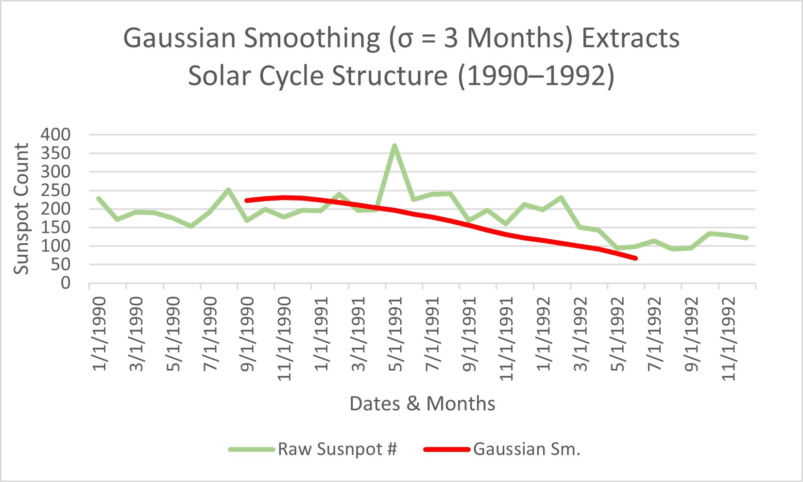
Data and Graphs of Solar Cycle 22A during periods of decline after the recent 1989 incident in Quebec before this timeline. (1990-1992)

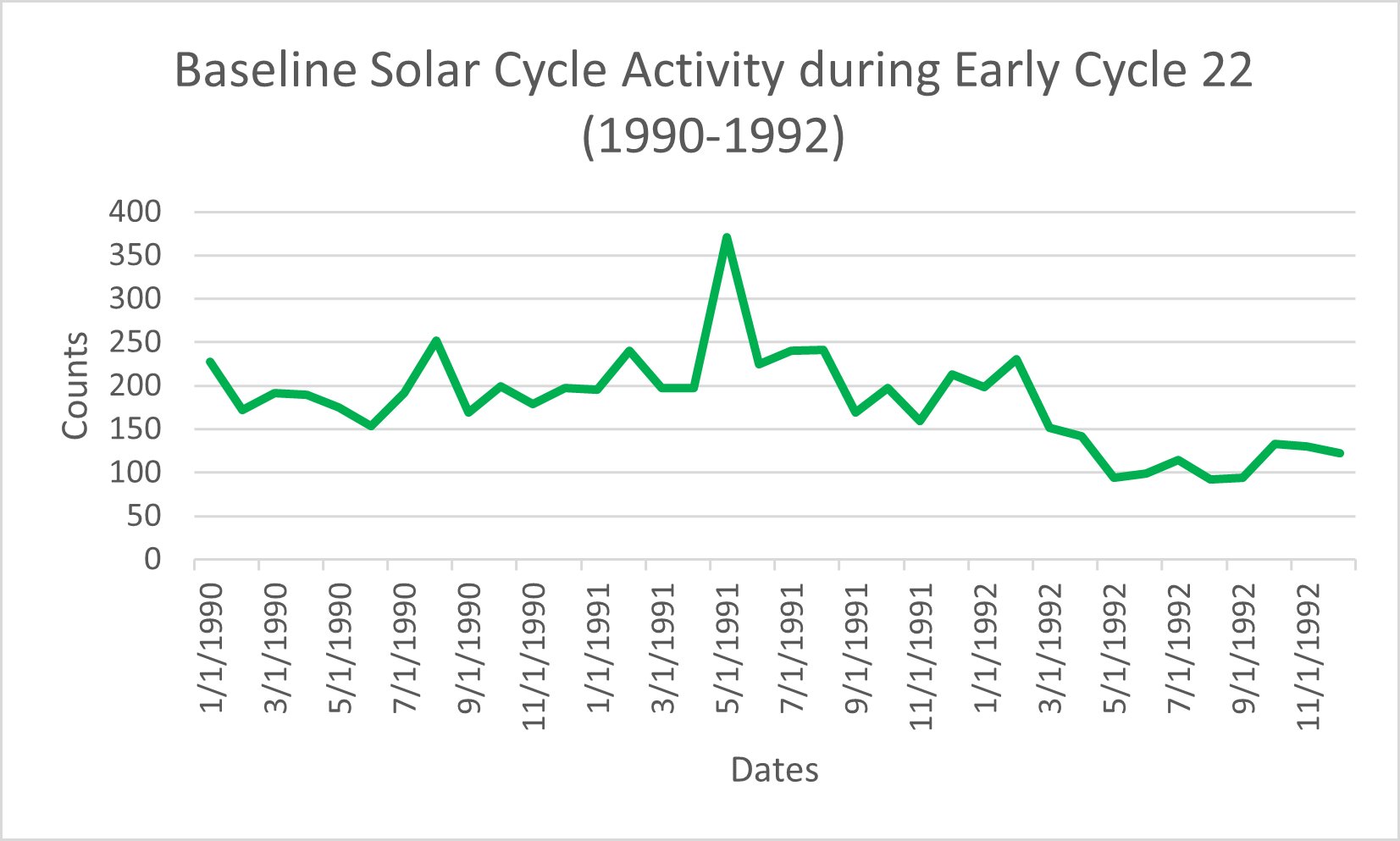Raw monthly sunspot numbers during 1990–1992 remain elevated, consistent with  the declining phase of Solar Cycle 22. While short-term fluctuations occur monthly, overall activity remains high, indicating sustained magnetic instability during this cycle segment. The 13-month smoothed average reduces short-term variability and clearly shows a gradual declining trend in sunspot activity. This confirms that although raw values fluctuate, the underlying cycle trend is slightly downward during this period.

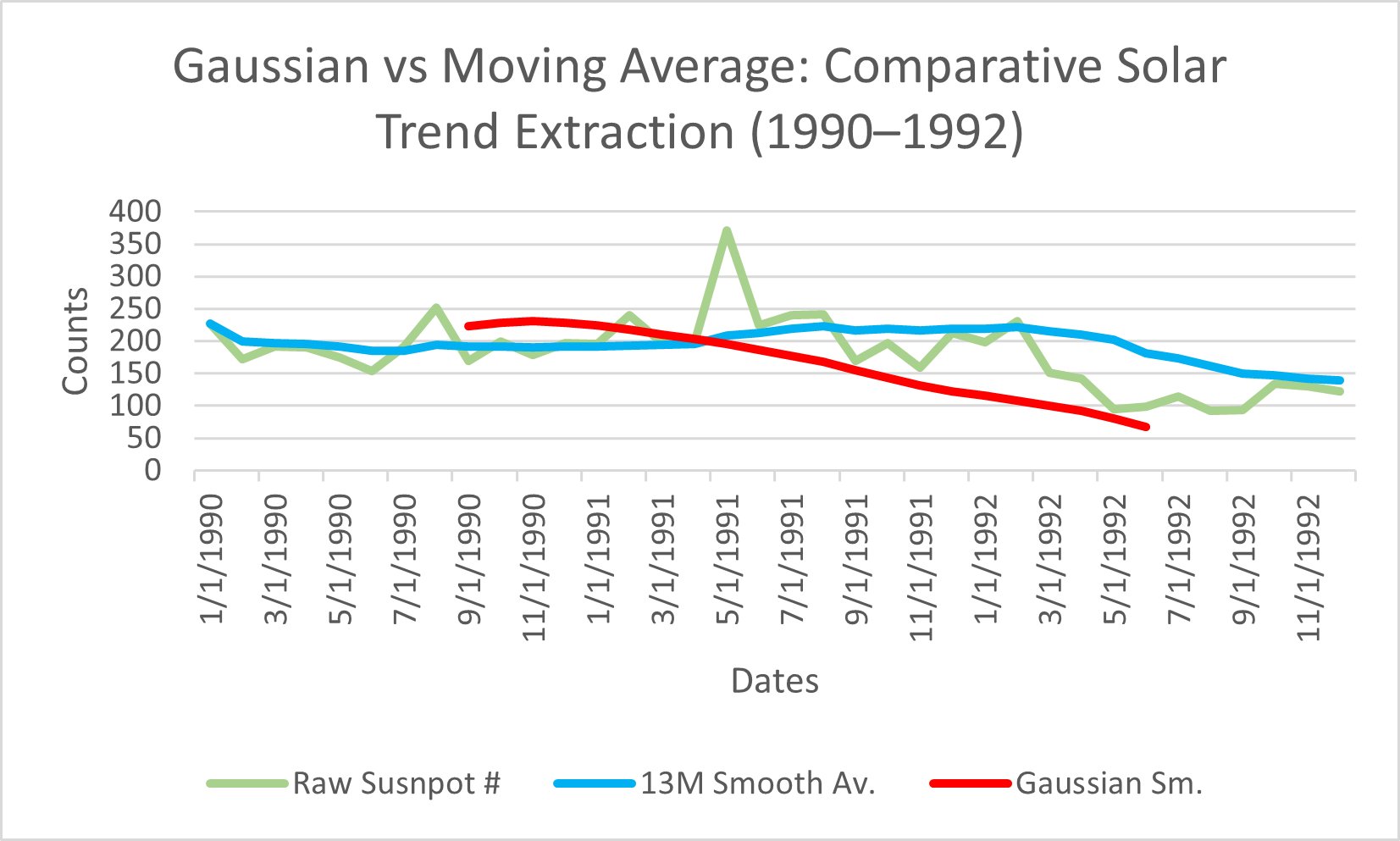
The Gaussian smoothing further refines the long-term trend by weighting nearby values more strongly. The resulting curve closely follows the smoothed average, reinforcing the gradual decline in solar activity from 1990 to 1992. Comparing raw sunspot numbers with smoothed data highlights the difference between short-term variability and long-term solar cycle behavior. The smoothing techniques reveal the underlying magnetic cycle progression more clearly than raw data alone. Summary: CME frequency shows a positive relationship with sunspot number during this period. Months with elevated sunspot activity correspond to increased CME occurrence, supporting the hypothesis that stronger magnetic complexity drives eruptive solar events.

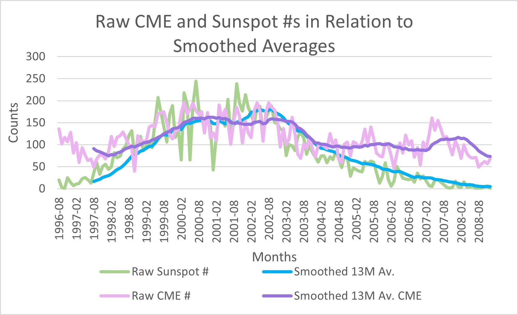
Full Cyclic Analysis of Solar Cycle 23, known as a rather puissant modern Solar Cycle. (1996-2008)

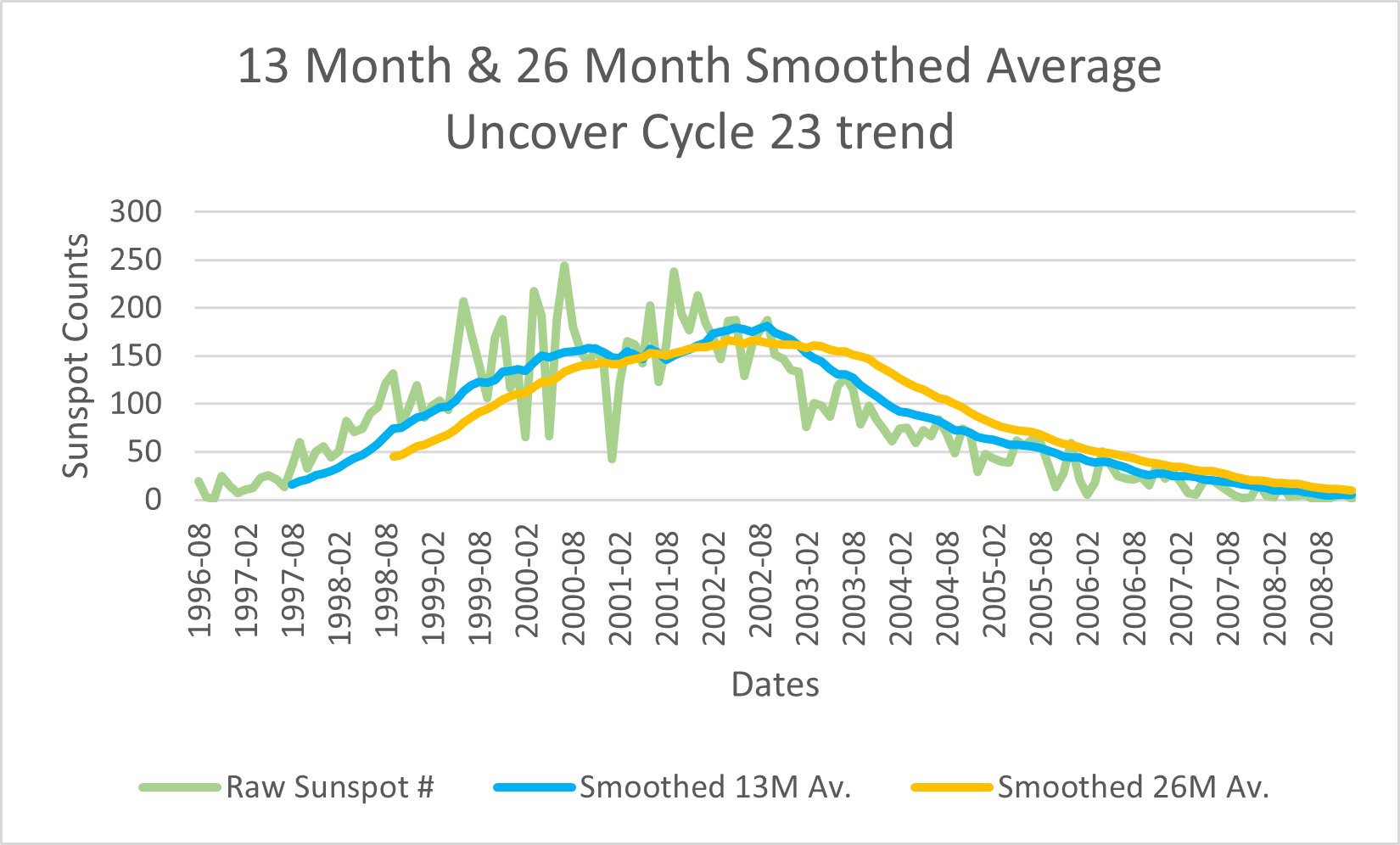
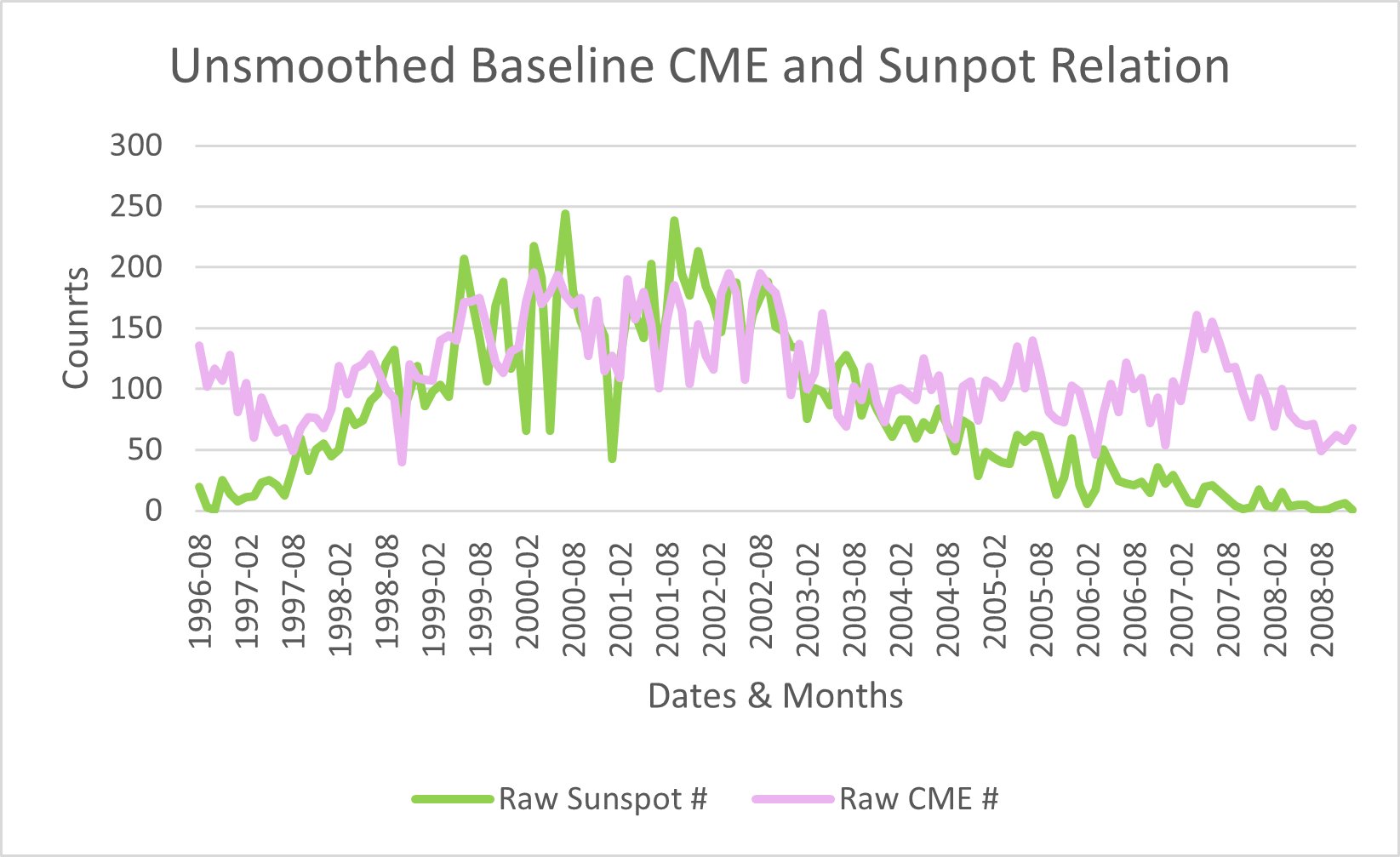As sunspot numbers increase during the rising phase of Solar Cycle 23, CME frequency also increases. The strengthening correlation indicates that active regions are becoming more magnetically unstable and eruption-prone. Furthermore, during the decline of Sunspot counts, CMEs don’t decline as drastically, displaying that CME activity remains relatively high even during periods of lower sunspot counts. 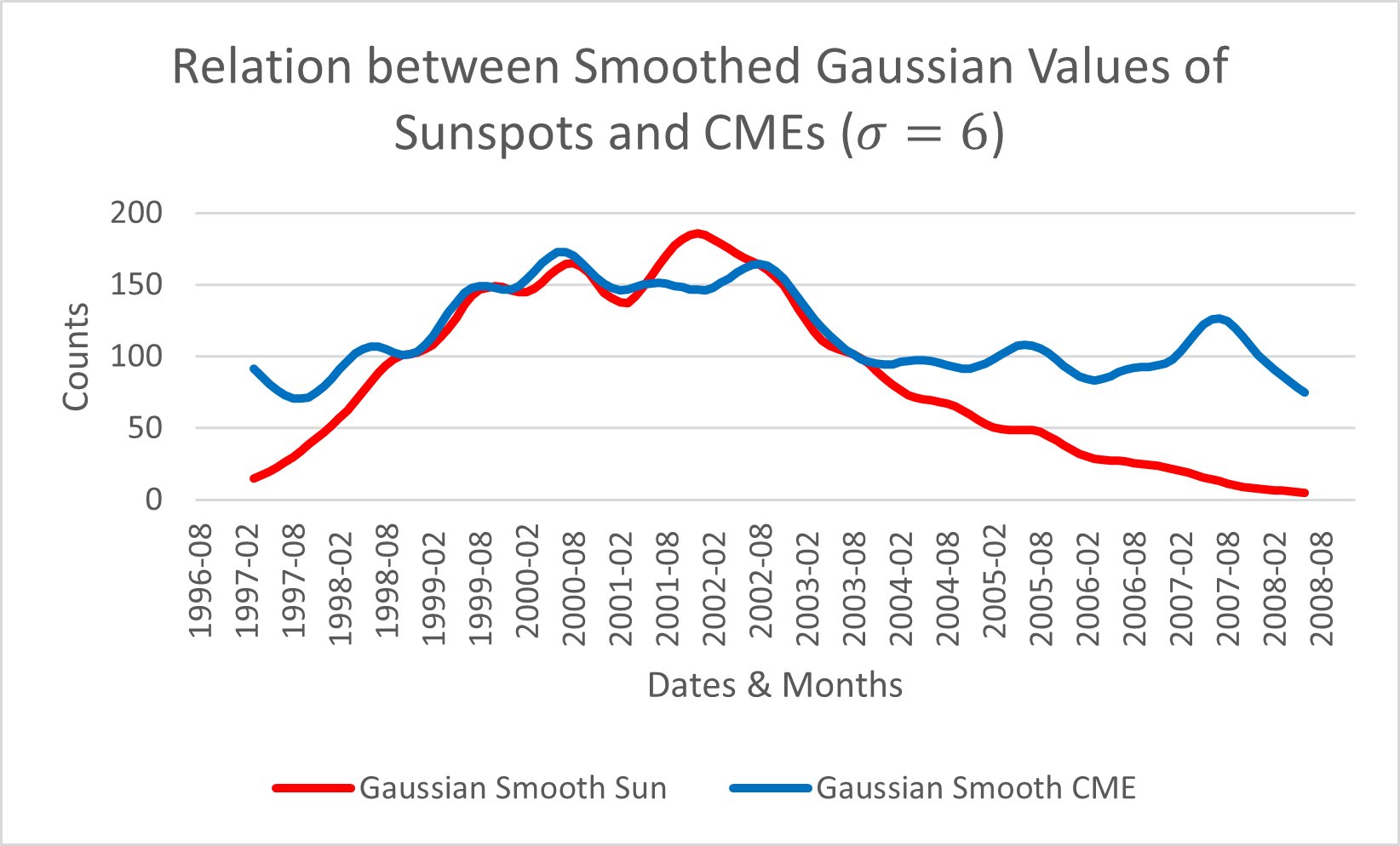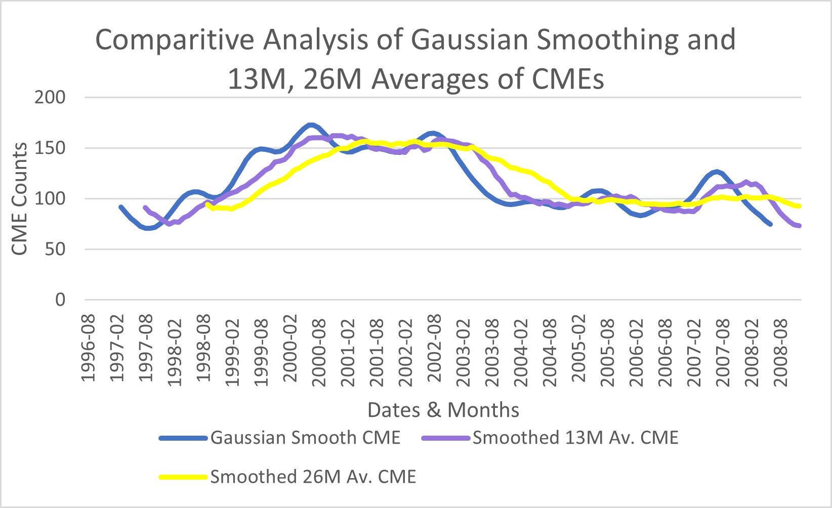The Gaussian Smoothing further refines the raw and Moving average counts of CMEs and sunspots by using weights to blur out edges. The resulting smoothed curve closely follows with the raw counts reinforcing the relationship mentioned above from 1996-2008. 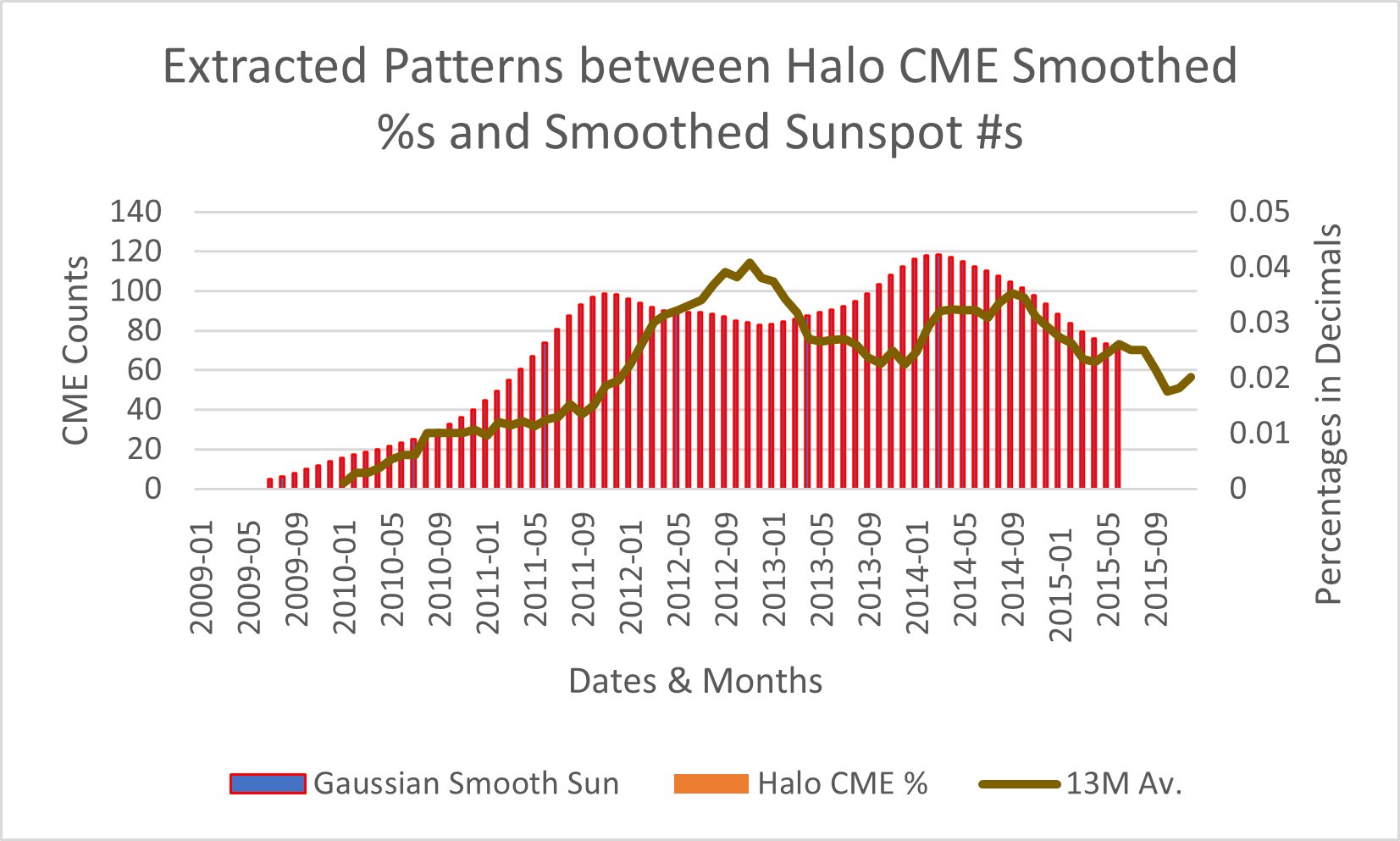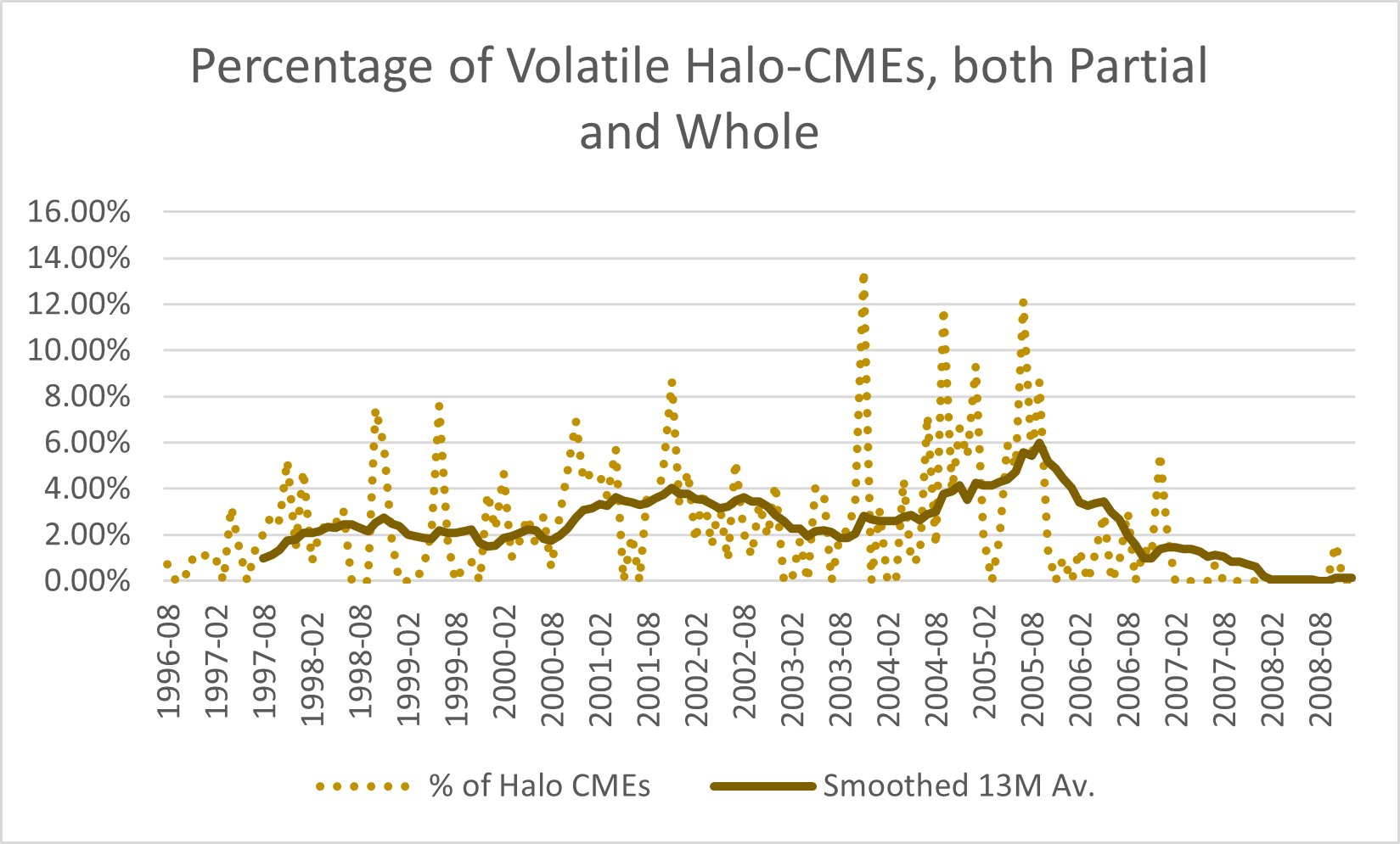Relationships and analysis of Smoothed Sunspot, CME counts in relation to volatile Halo-CMEs show that both scale linearly as dictated by the solar cycle. However, spikes in Halo-CME percentage during August 2005 is a limitation, as with a lower overall CME count, even a moderate Halo CME count could make Halo percentage spike, causing occasional false warnings in devices utilizing this data. 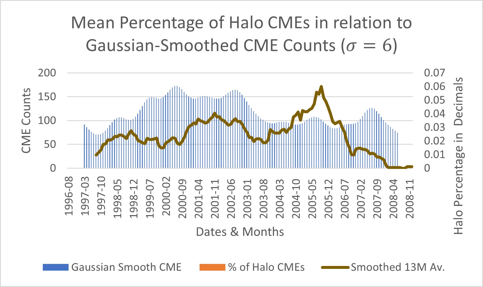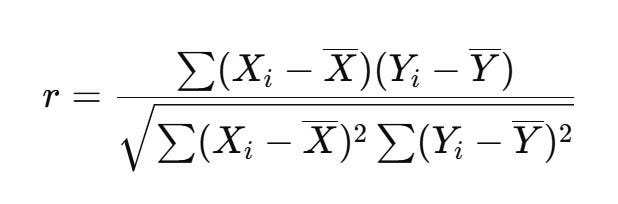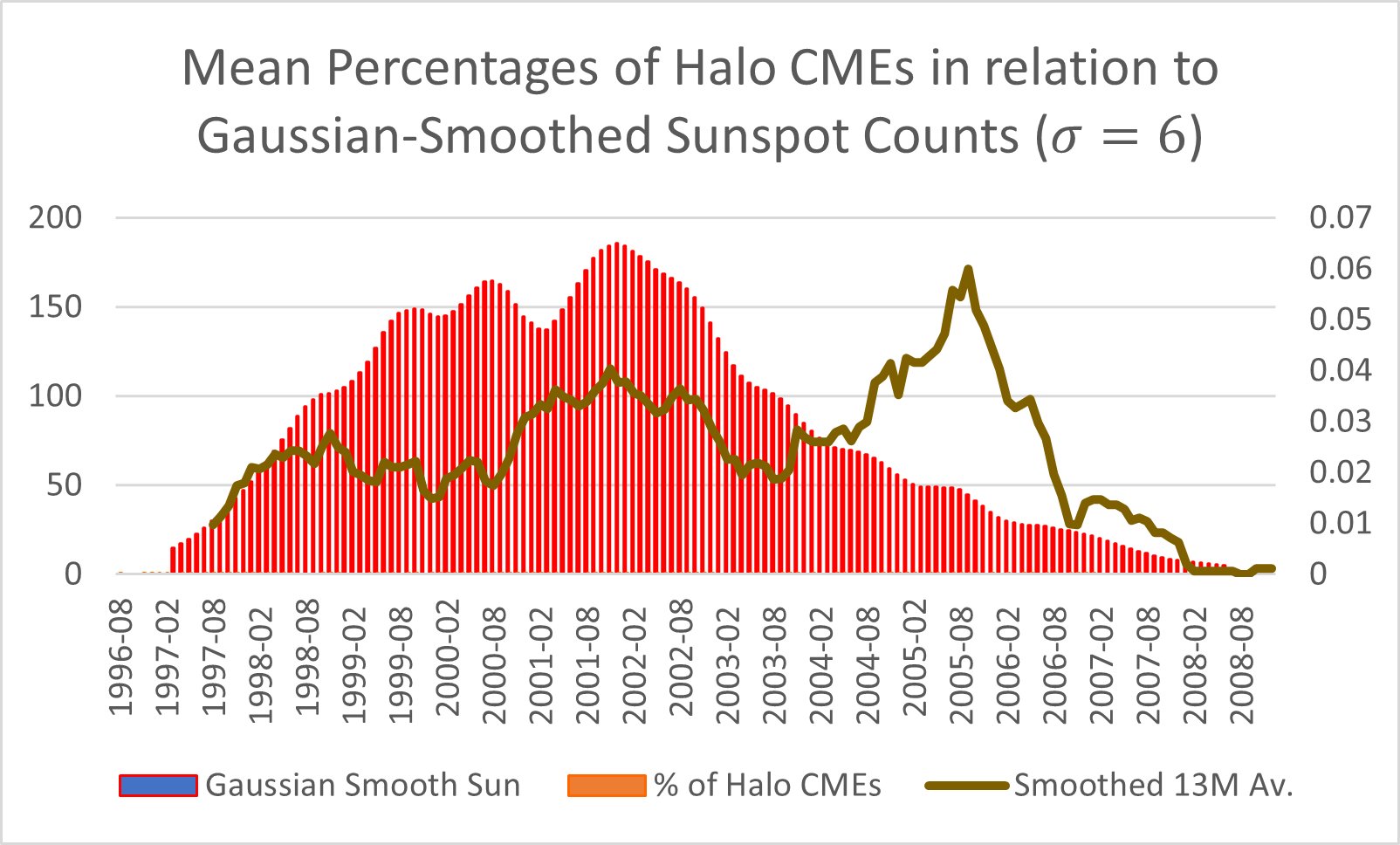The Mean Percentages of Halo CMEs to Gaussian smoothed Sunspot or CME counts show the relationships that Halo chances have in relation to these parameters. Even though after applying the Pearson Correlation Coefficient, the correlation comes out to be 1.3 or weak, generally Halo percentages grow and decline with CME percentages. The skewing of the correlation maybe a byproduct of the extreme Halo Percentage peak from August 2004 to August 2006, when magnetic activity was in the phase of decline. Formula for Pearson Correlation Coefficient:

Summary: CME frequency shows a positive relationship with sunspot number during this period. Months with elevated sunspot activity correspond to increased CME occurrence, supporting the hypothesis that stronger magnetic complexity drives eruptive solar events.

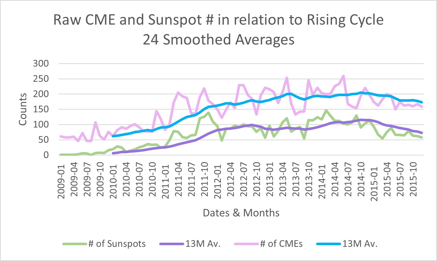
Analysis of Cycle 24 rising solar activity dynamics with extreme minima periods and one of the lowest solar activity not including the Maunder Minimum Period

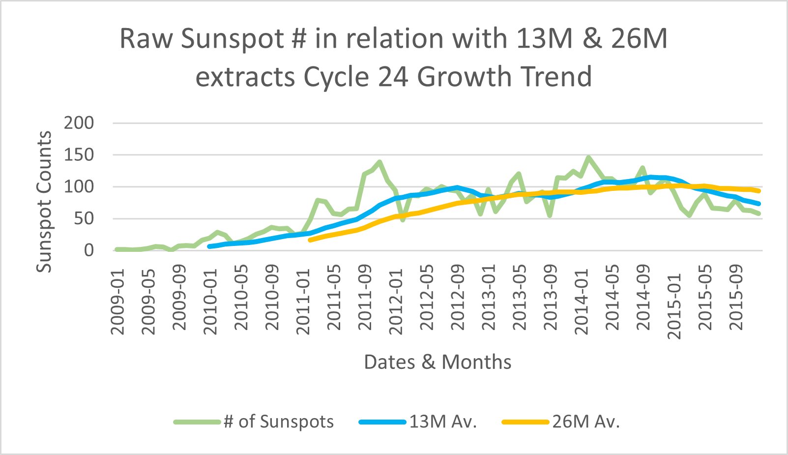
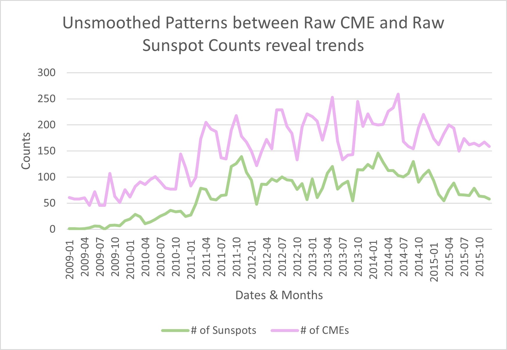As sunspot numbers increase during the rising phase of Solar Cycle 23, CME frequency also increases. The strengthening correlation shows that changes in sunspot count throughout  2009-2015 are well justified by equivalent changes in CMEs. The smoothed 13-month average of sunspot occurrences show that even though sunspots have a positive correlation with CMEs, solar activity was passive and stagnant, creating a deep minima period.

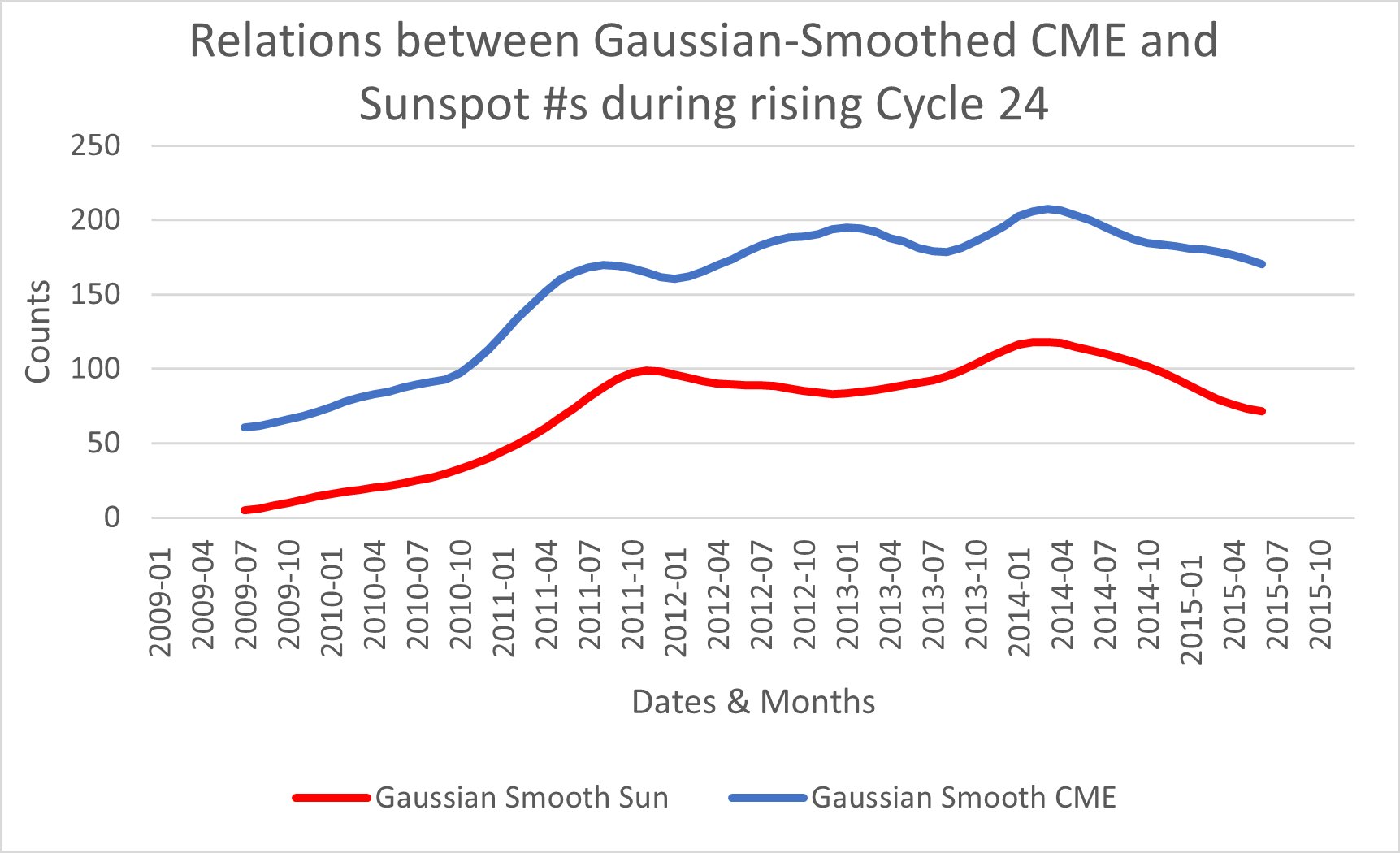
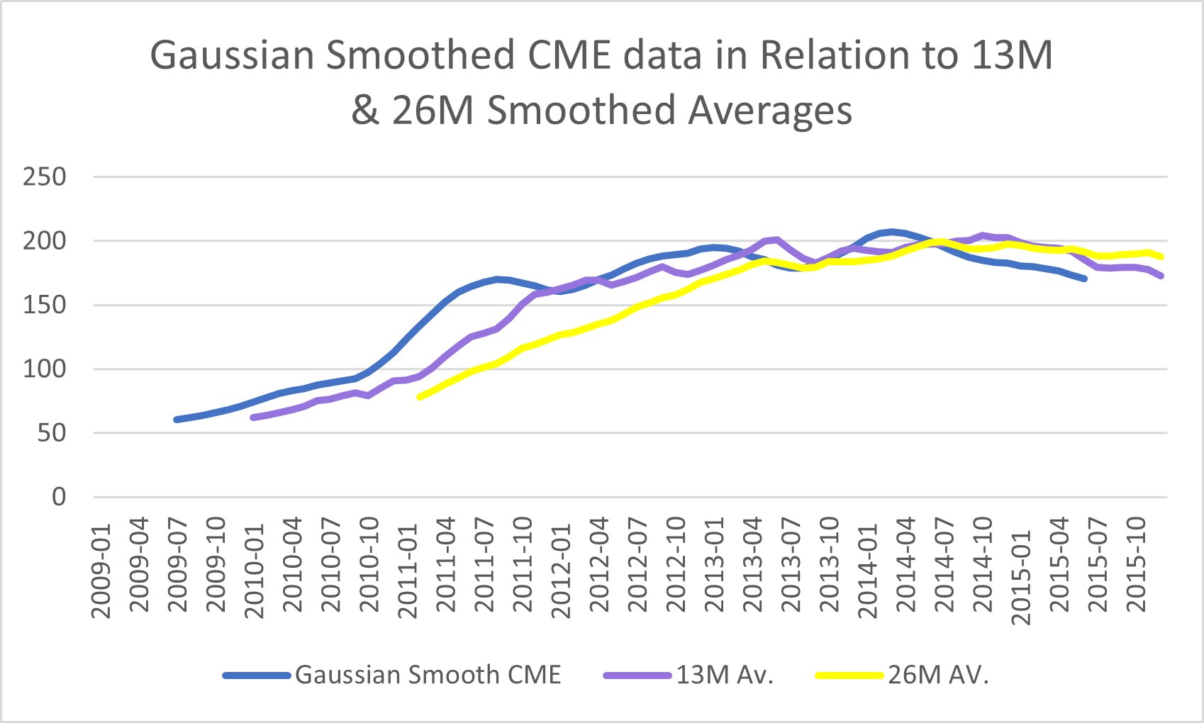
The Gaussian Smoothing further deletes the raw noise provided by the moving average and the monthly counts. This smoothing helps to dig further into the correlations of CMEs and Sunspots. Even with heavy smoothing, Gaussian Smoothing preserves the high correlation seen in CME and Sunspots. However, between Jul 2010 and Oct 2011, the Gaussian smoothing further increases than both the moving averages only to meet in Jan 2012. A similar pattern can be noticed when comparing the 13-month smoothing to the 26-month smoothing. Displaying a possible bubbling pattern between varying smoothed averages and Gaussian smoothing weights. 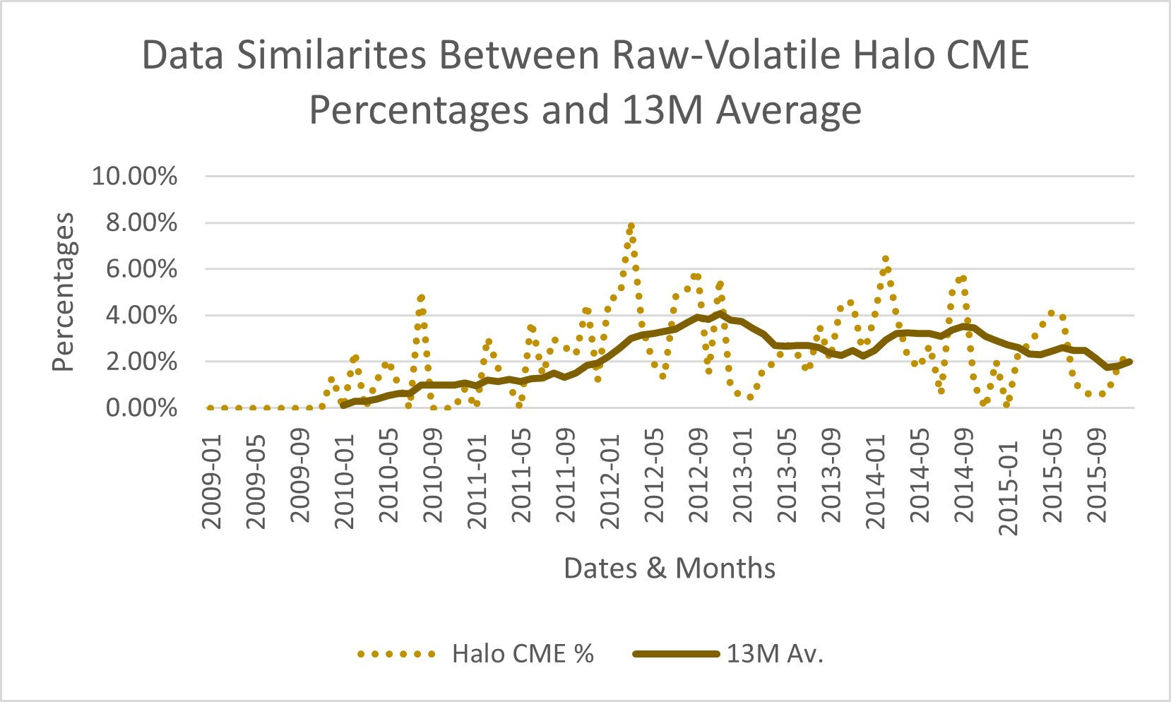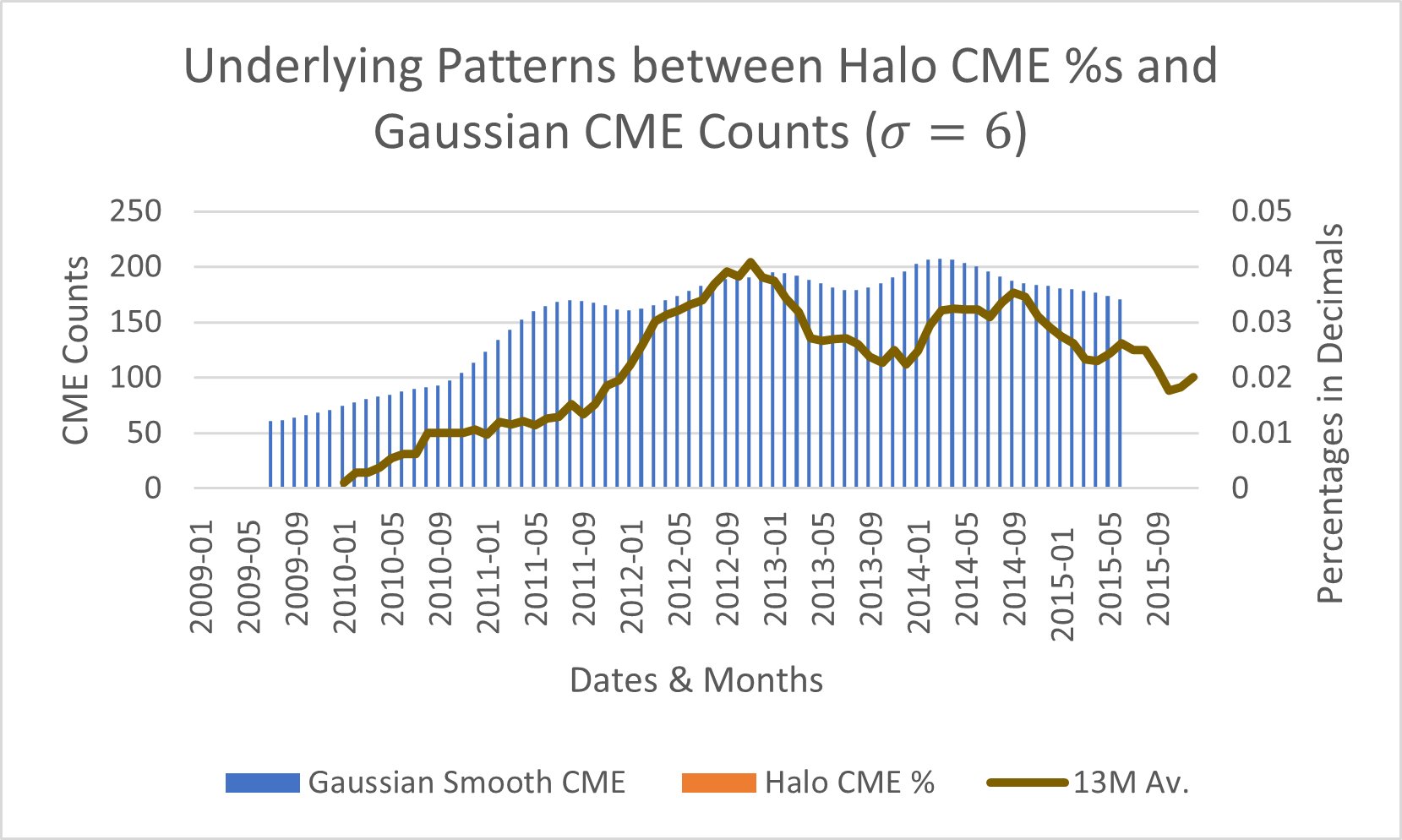The Mean Percentages of Halo CMEs to Gaussian smoothed Sunspot or CME counts show that Halo percentages in Solar Cycle 24 scale linearly with CME and sunspot occurrences. Upon calculating the Pearson Correlation Coefficient using,

The correlation comes out to be 0.86 which is categorized as a positive correlation where 73.96% of changes in each variable is justified by the other. This mathematical computation shows that with increasing CME occurrences, chances of Halo-CMEs also  increase in a similar pattern especially during periods with deep minima and low solar activity. As seen in Solar Cycle 23, CME occurrences and Halo CME occurrences go hand-in-hand during the early and Rising periods of a Solar cycle explaining the anomaly in which Halo-CME activity peaked in Late-Cycle 23. Summary: Although Solar Cycle 24 exhibits lower overall sunspot values, the positive correlation between sunspot number and CME count remains evident. This suggests that even weaker cycles maintain the same fundamental magnetic eruption mechanism.

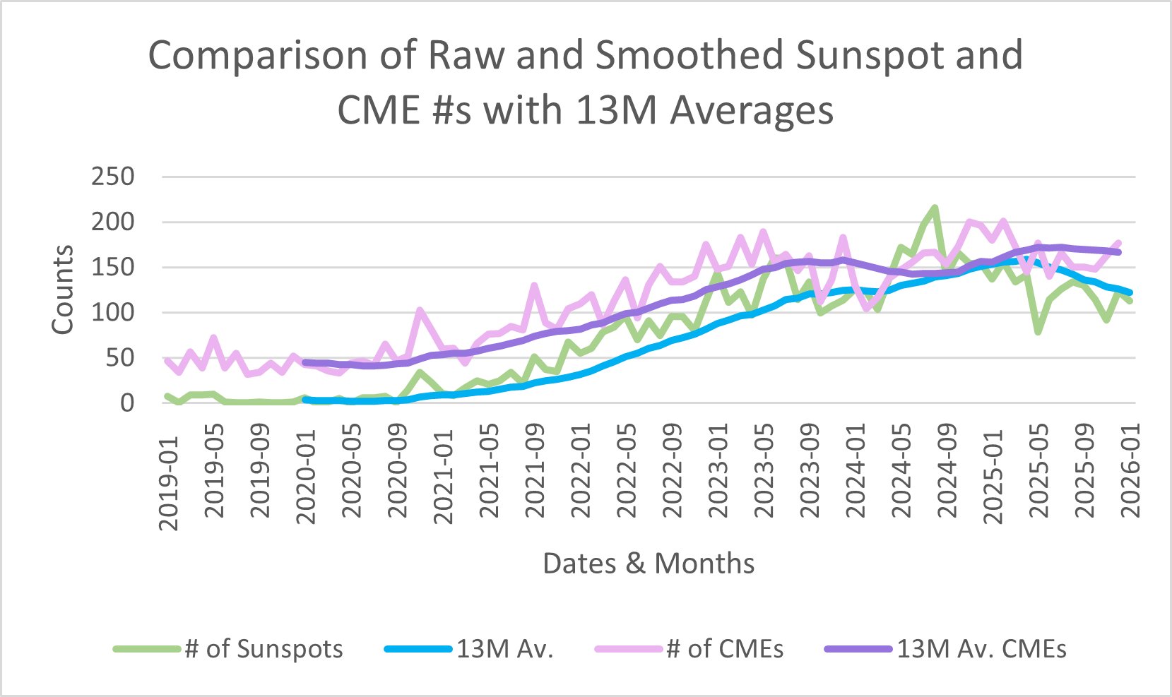
An in-depth extraction of data for the most recent Solar cycle with high solar activity, a part of the recent Modern Maxima. Solar Cycle 25 (2019-2026)

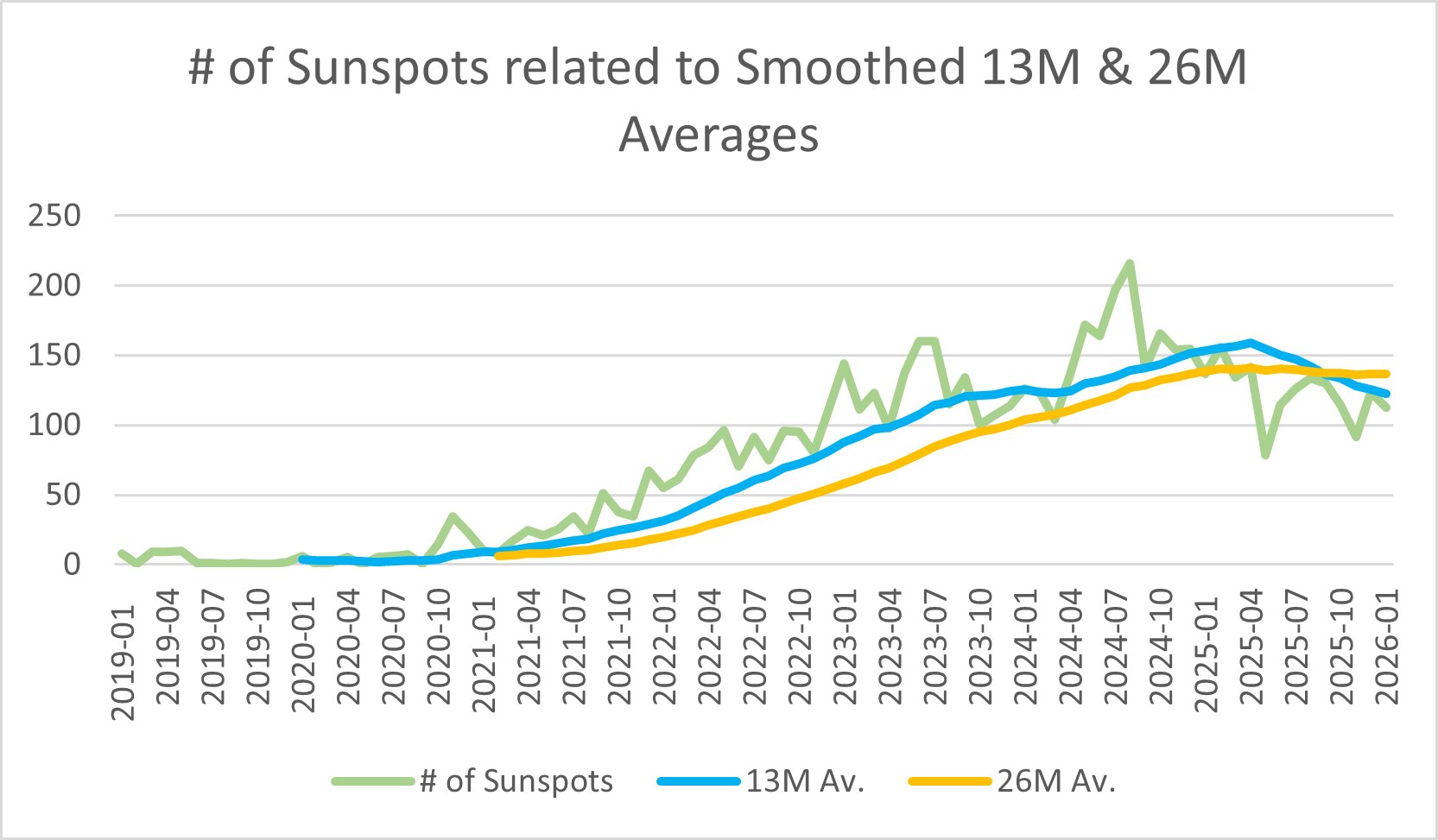
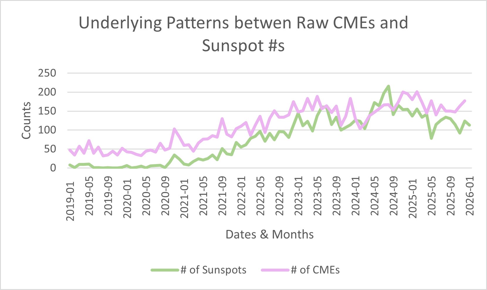As sunspot numbers increase during the rising phase of Solar Cycle 23, CME frequency also increases. The strengthening correlation shows that changes in sunspot count throughout  2019-2026 are well justified by equivalent changes in CMEs. The smoothed 13-month average of sunspot occurrences show that even though sunspots have a positive correlation with CMEs, solar activity was active and higher than solar cycle 24 with peak sunspot counts of 210 highlighting a stronger rebound after Solar Cycle 24.

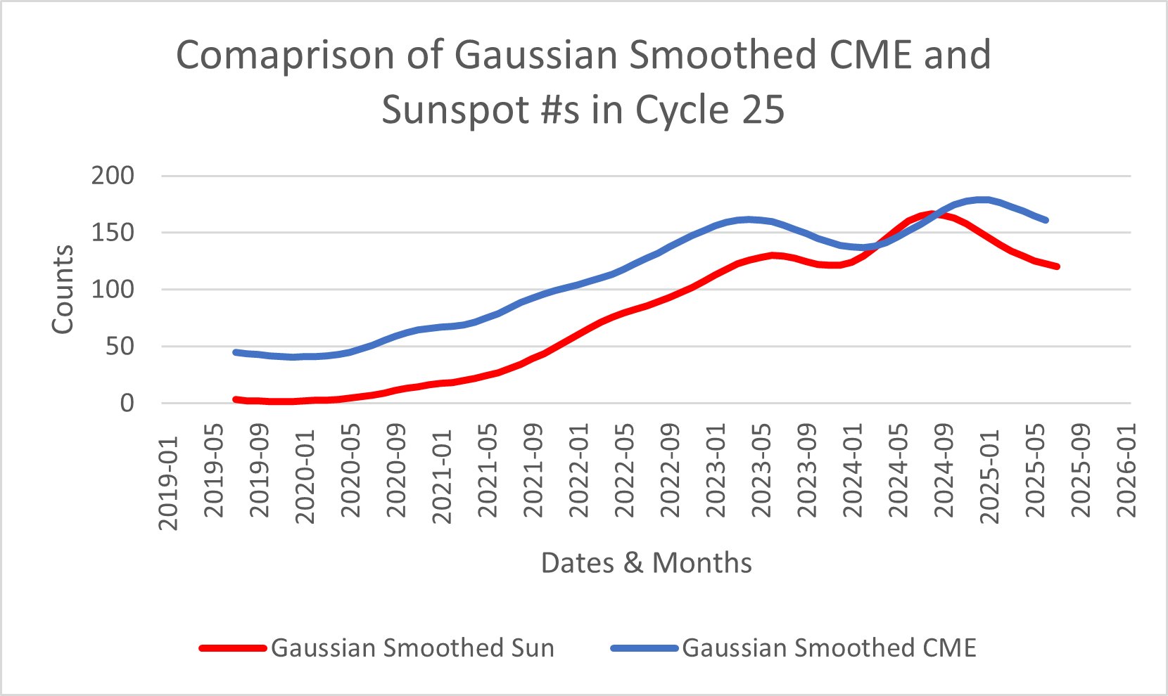
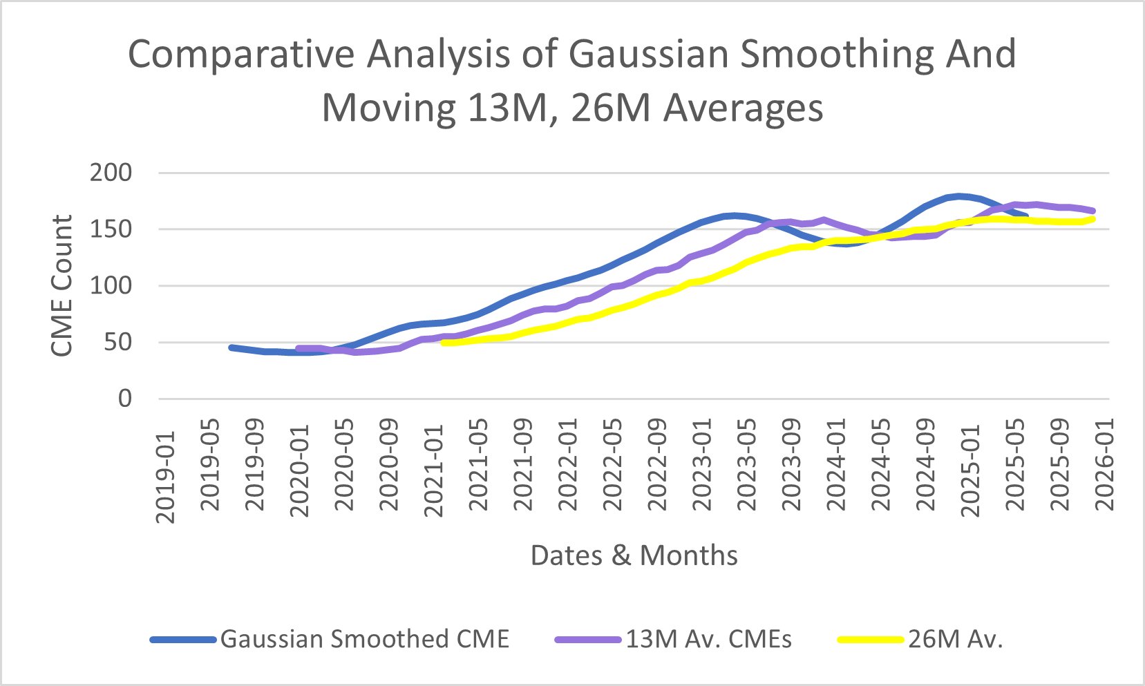
The Gaussian Smoothing further deletes the raw noise provided by the moving average and the monthly counts. This smoothing helps to dig further into the correlations of CMEs and Sunspots. Even with heavy smoothing of σ=6, Gaussian Smoothing preserves the high correlation seen in CME and Sunspots. However, there is a slight lag between the 13-month average of CME as a dip in CME occurrences is during Feb 2024 for Gaussian smoothed counts, while in 13-month smoothed average, it dips in Sep 2024. This displays occasional mismatches between Gaussian blurring and moving averages proving as a limitation for CME prediction & pattern-hunting.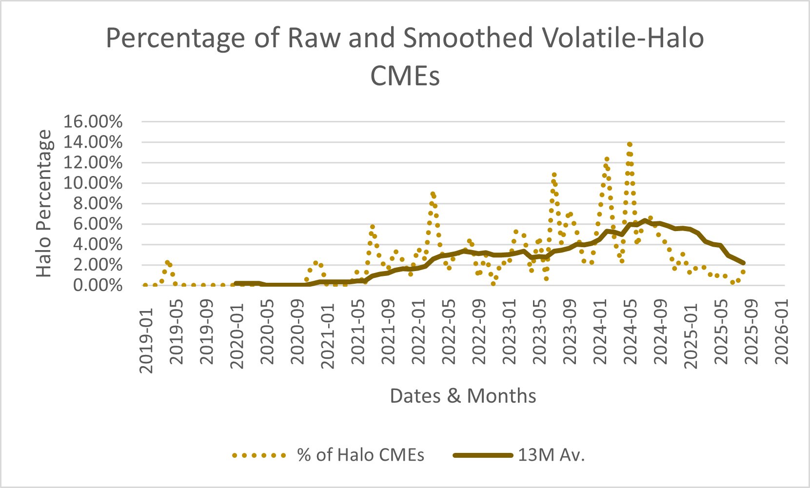 Relationships between the gradual increase of CME Count and  Volatile Halo CME Count reveals an underlying shared driving force between both circumstances. The Volatile Halo-CME Count peaks in May 2024 while CME and Sunspot Activity peaked later during Oct 2024 creating an approximate lag of 5 months, which shows that Halo-CMEs peak before CME occurrences as to increase CME percentage a moderate total CME count would be optimal which cannot happen during high CME Count. 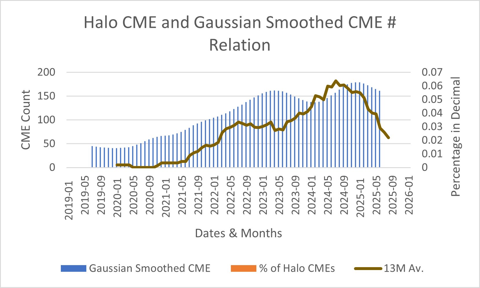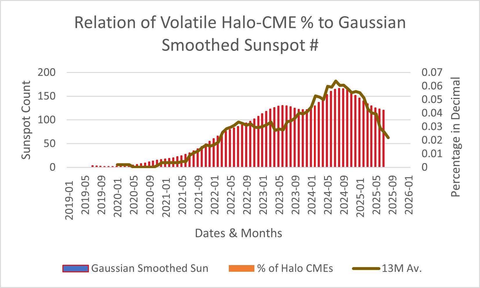The Mean Percentages of Halo CMEs to Gaussian smoothed Sunspot or CME counts show that Halo percentages in Solar Cycle 24 scale linearly with CME and sunspot occurrences. Upon calculating the Pearson Correlation Coefficient using the formula above. The correlation comes out to be 0.89 which is categorized as an extremely positive correlation where 79.21% of changes in each variable is justified by the other. This mathematical computation shows that with increasing CME occurrences, chances of Halo-CMEs also increase in a similar pattern especially during periods with deep minima and low solar activity. However, the relation between CMEs and sunspots shifts during periods of extremely high Solar activity similar to Solar Cycle 23’s high mismatch between CME and sunspot counts, showing that high solar activity decreases correlation between Halo-CMEs and CME occurrences. Summary: During the early rise of Solar Cycle 25, increasing sunspot activity corresponds with rising CME frequency. This reinforces the consistency of the sunspot–CME relationship across multiple solar cycles.

Extracting patterns during an off-cyclic burst during November 2011

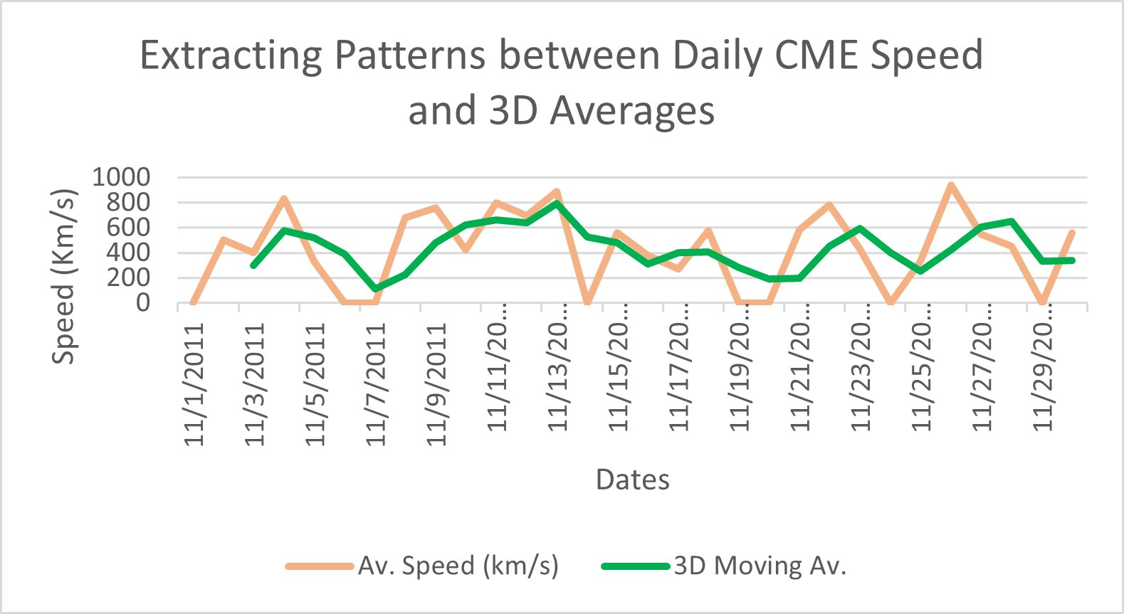
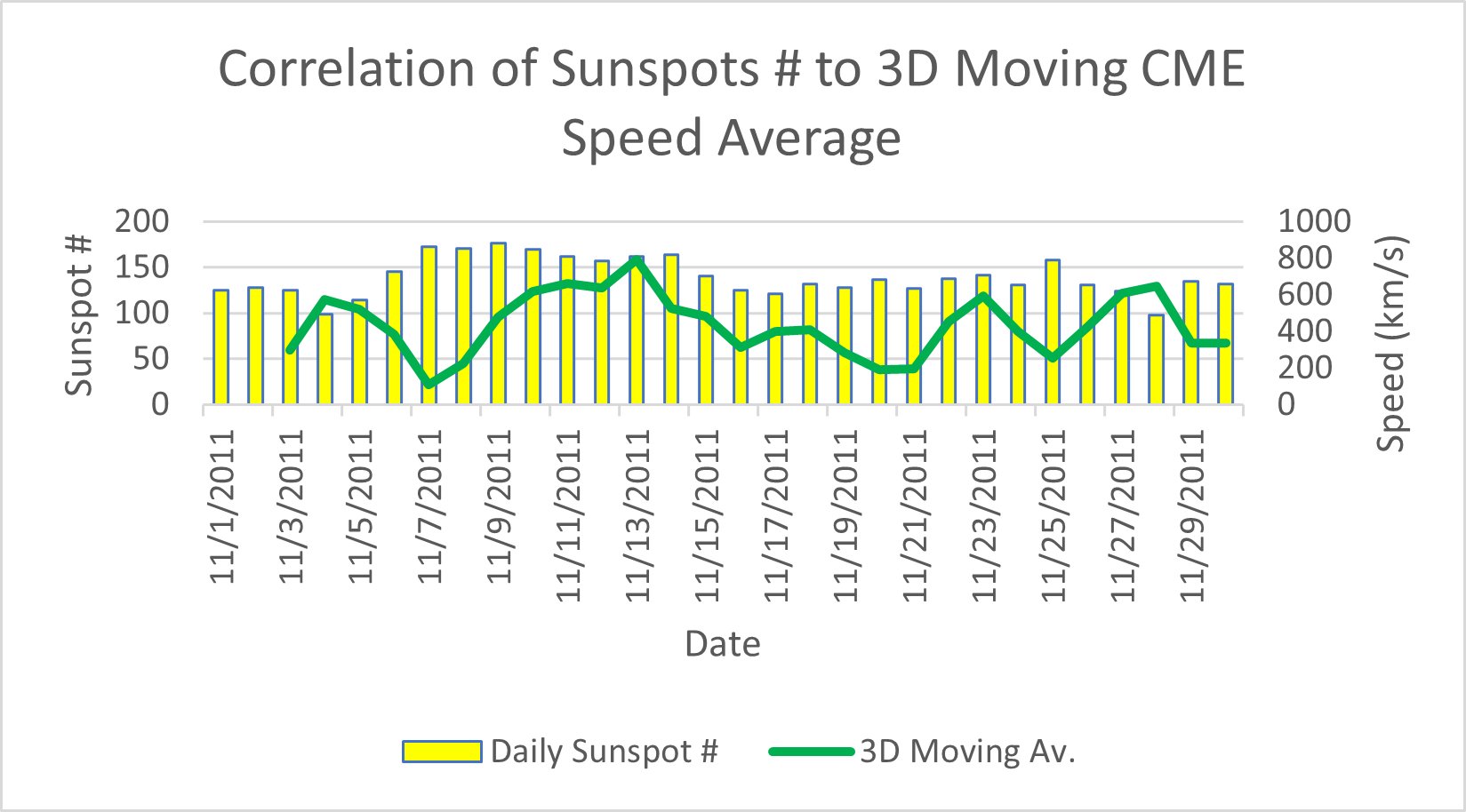
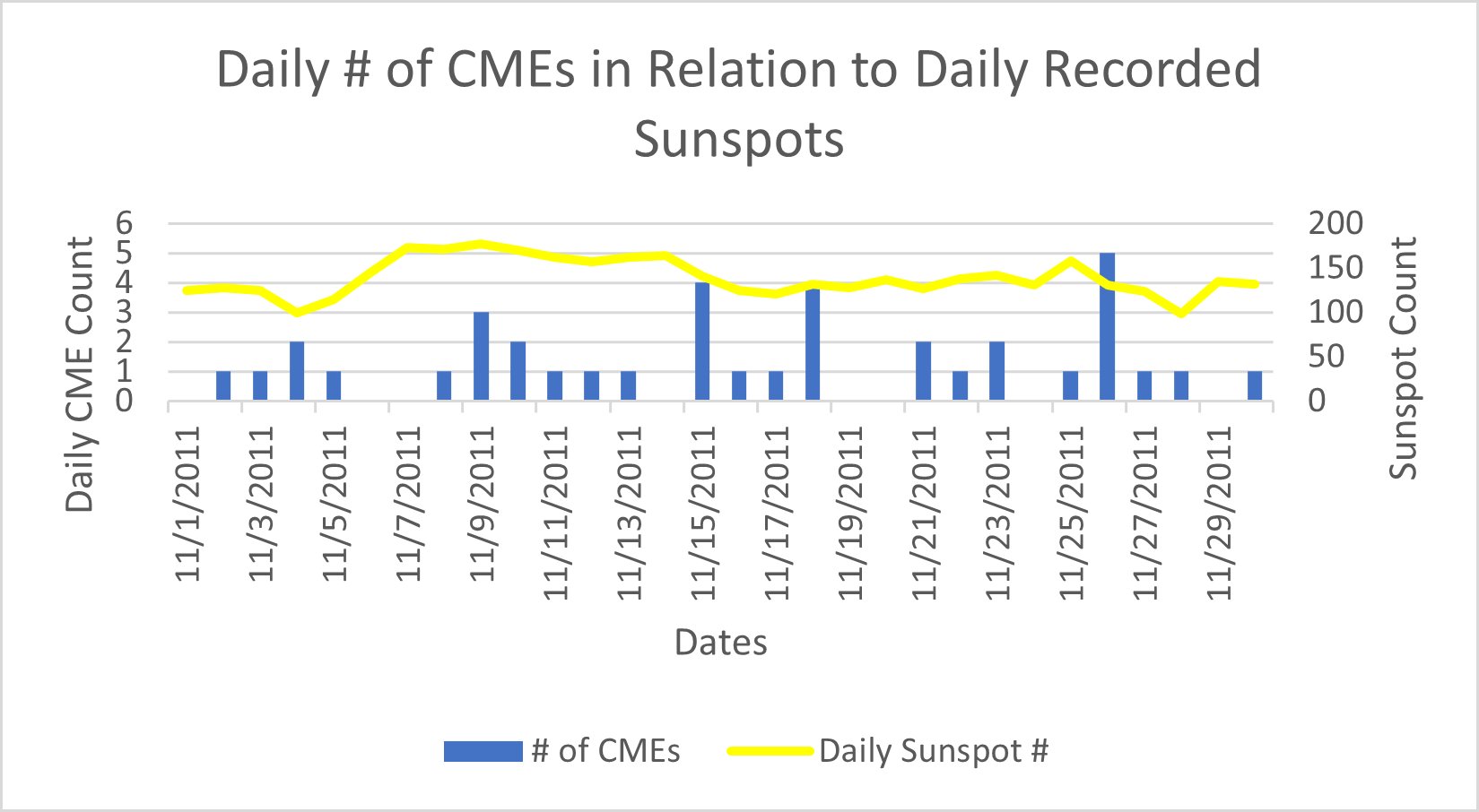
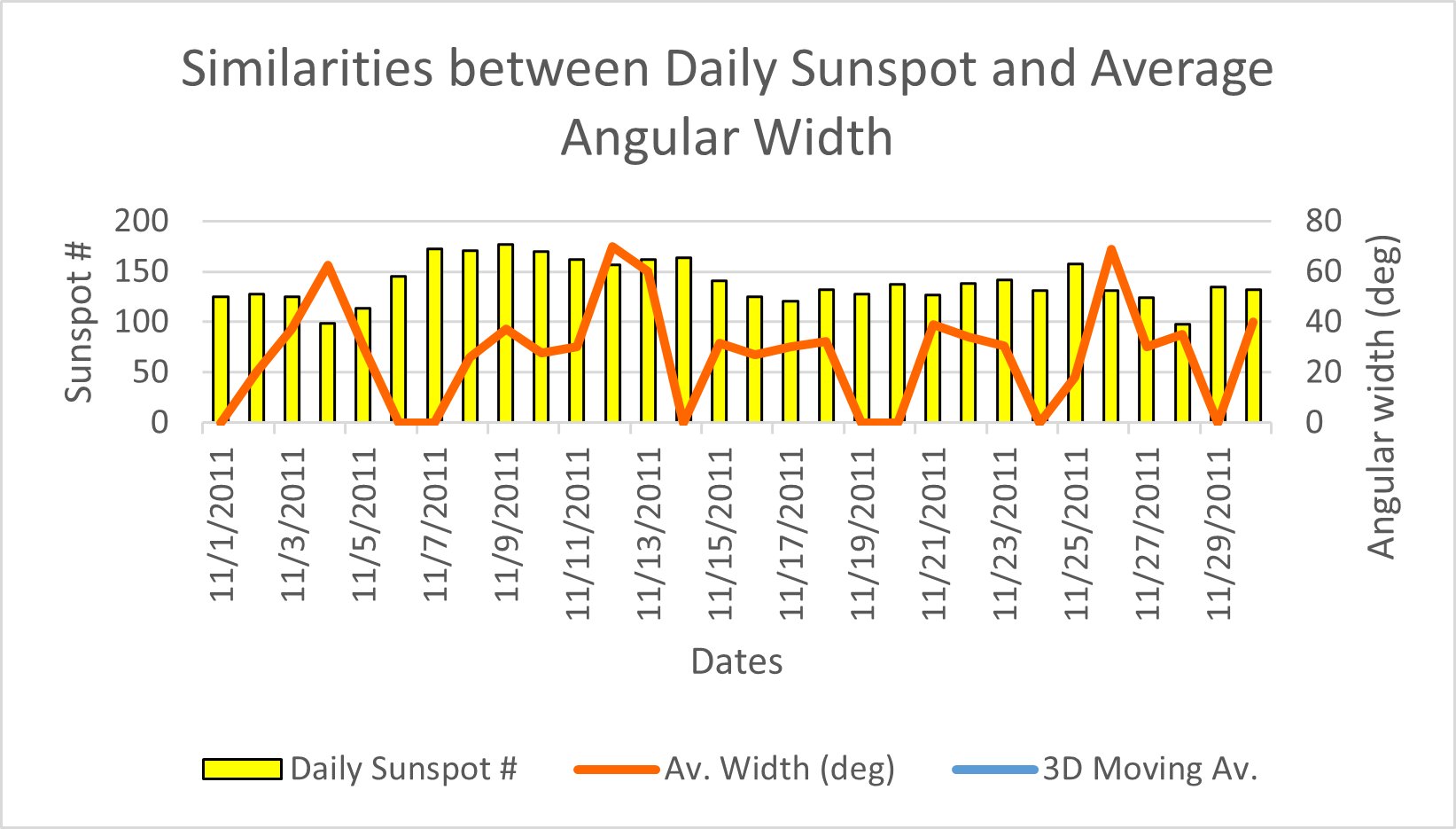
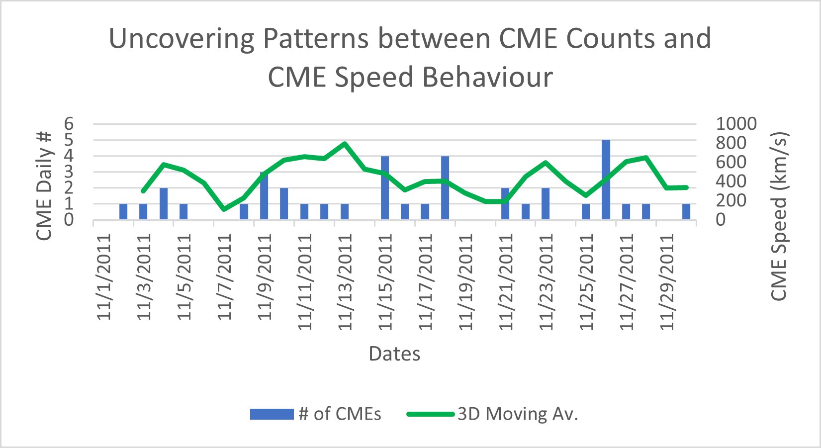
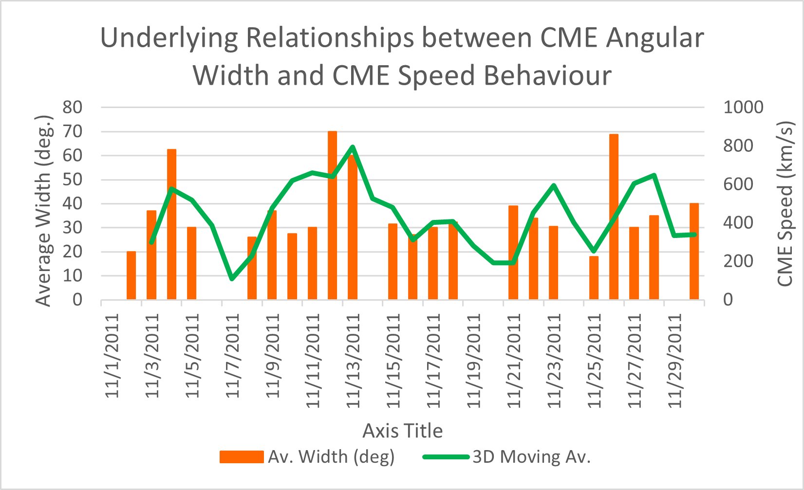The November 2011 burst shows a sharp increase in CME activity corresponding to elevated sunspot numbers. This supports the hypothesis that intense magnetic regions increase the probability of major eruptive events.

Hunting Correlations during September 2017 off-cycle local maximum with unusually high average CME speeds

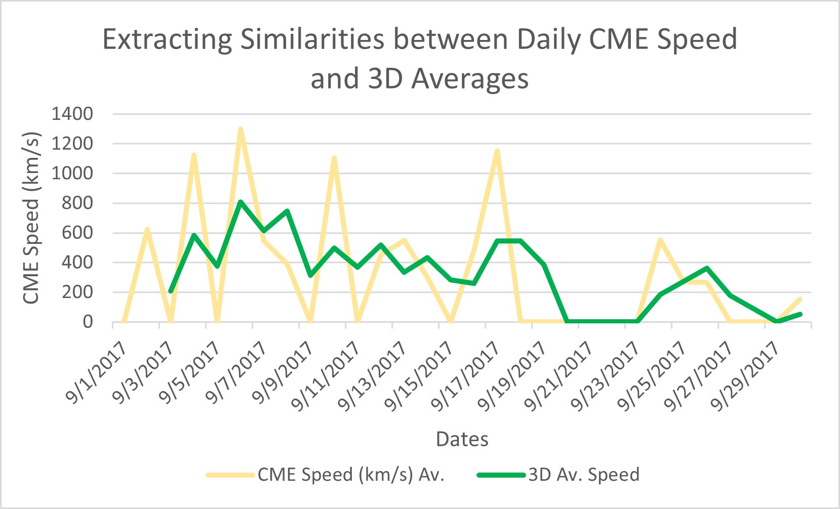
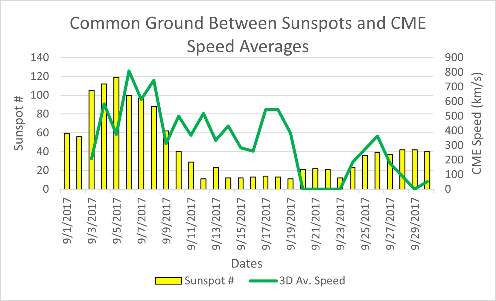
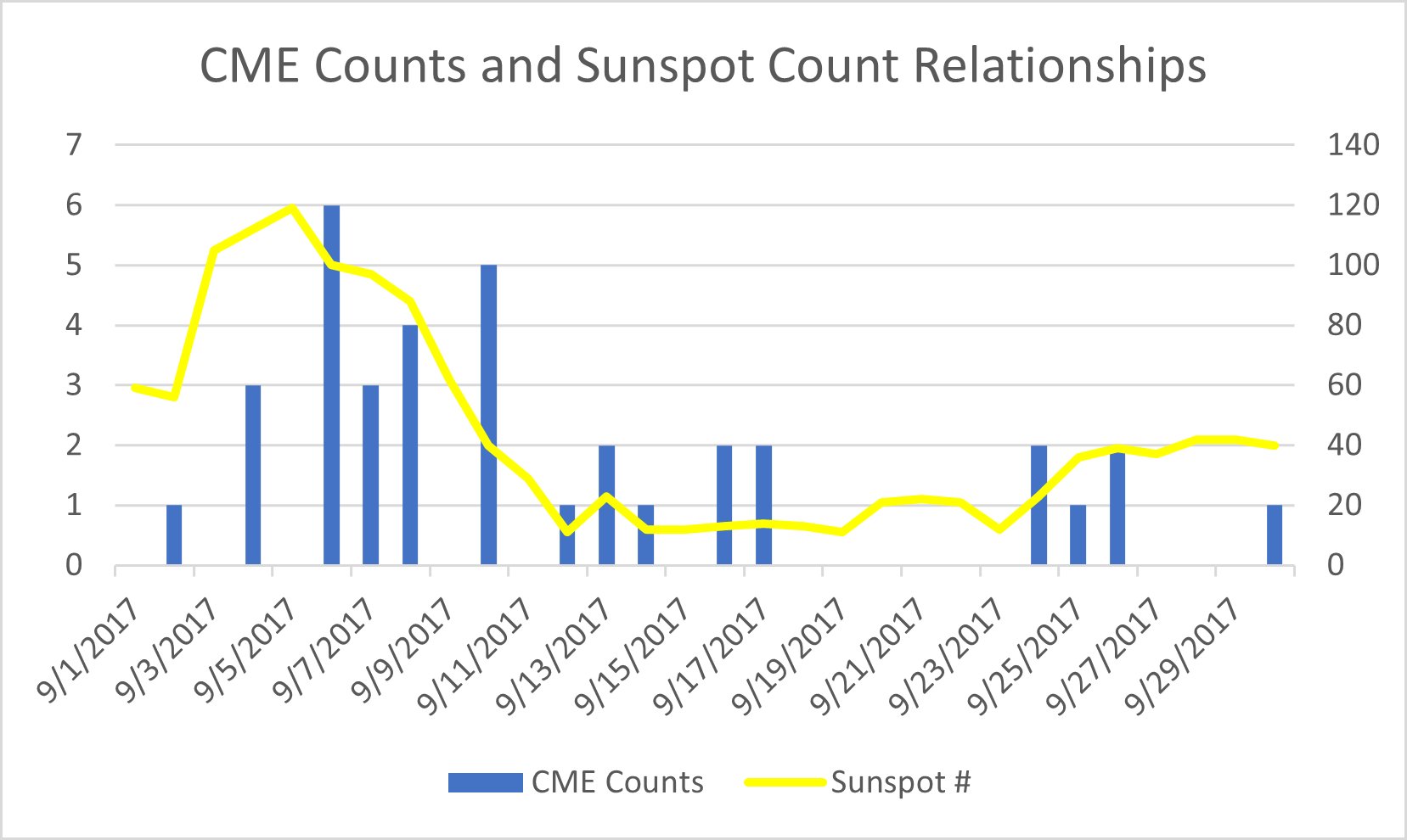
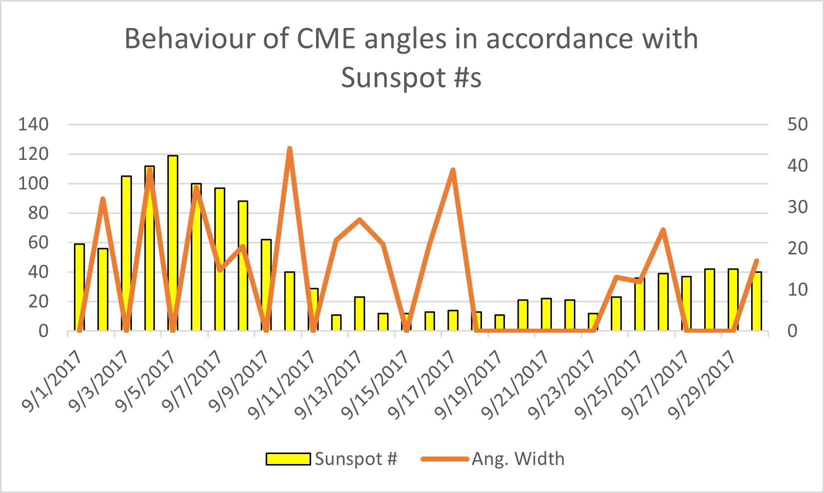
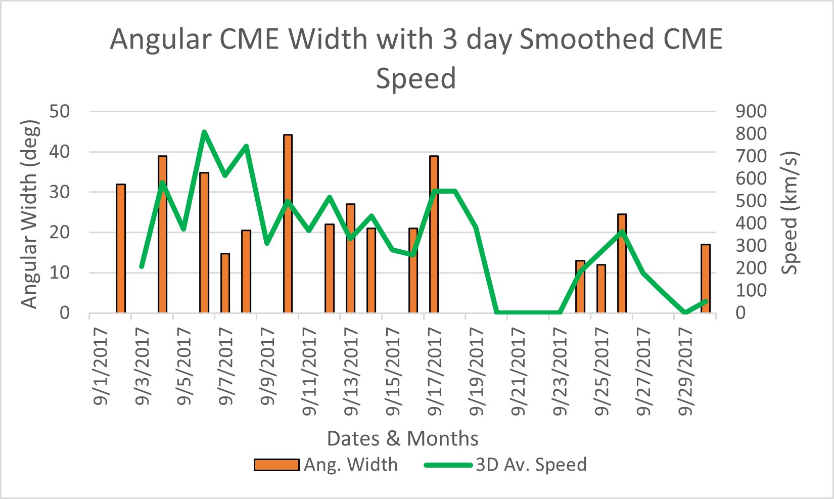
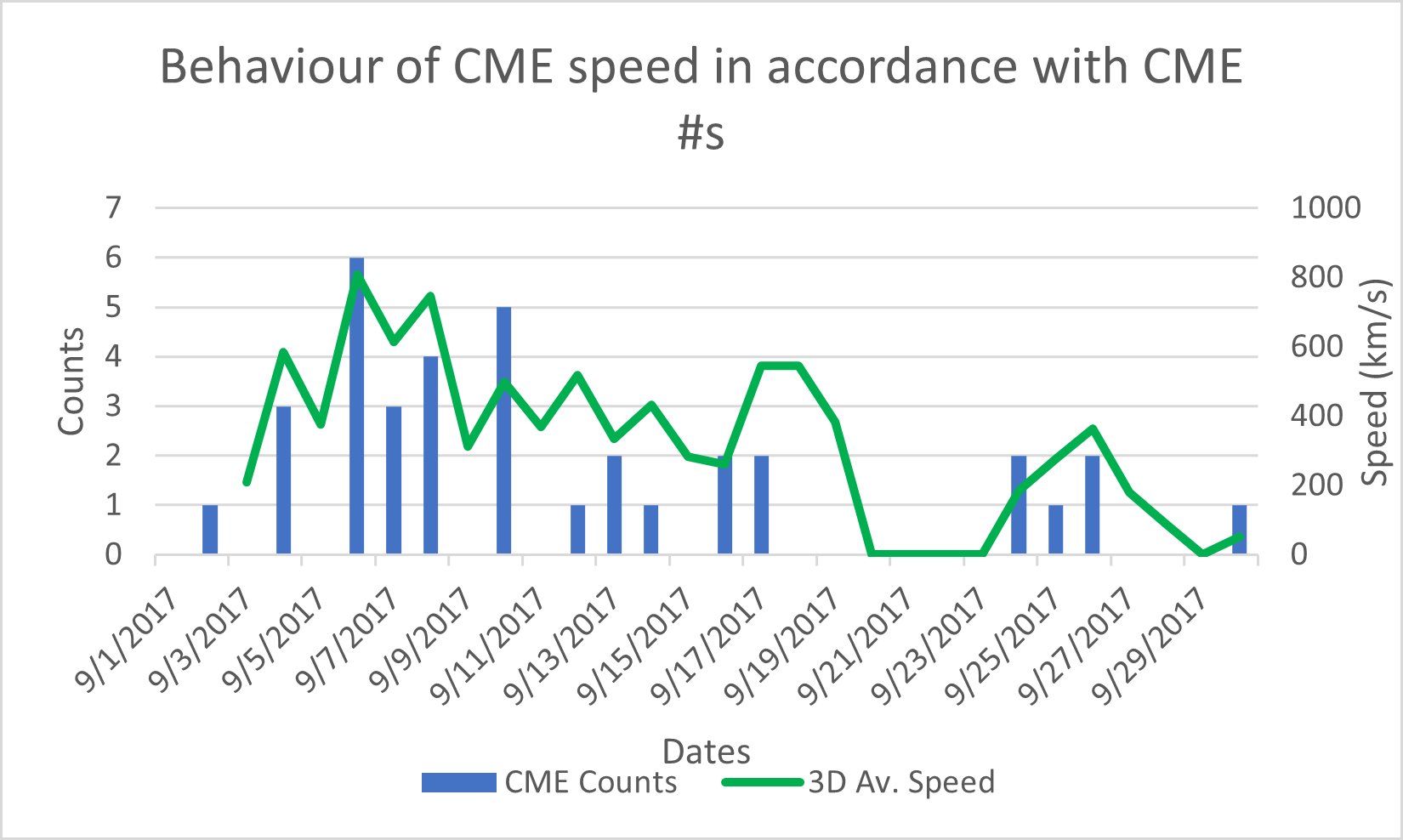The September 2017 event represents a late-cycle surge in activity. Although Solar Cycle 24 was declining, localized magnetic reconnection triggered significant CME production. This shows that off-cycle CMEs are common in weak cycles, and Halo-guided CMEs do not scale linearly with Maxima of Minima periods.

July 2012 CME activity peak with unusual burst severity highlighted with events at par in potential damage to the infamous 1859 Carrington Event.

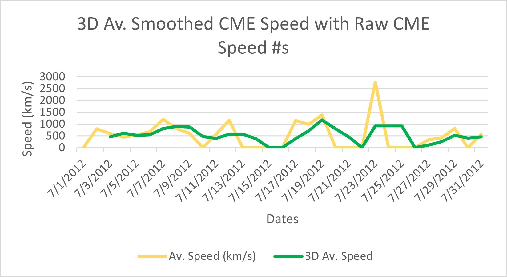
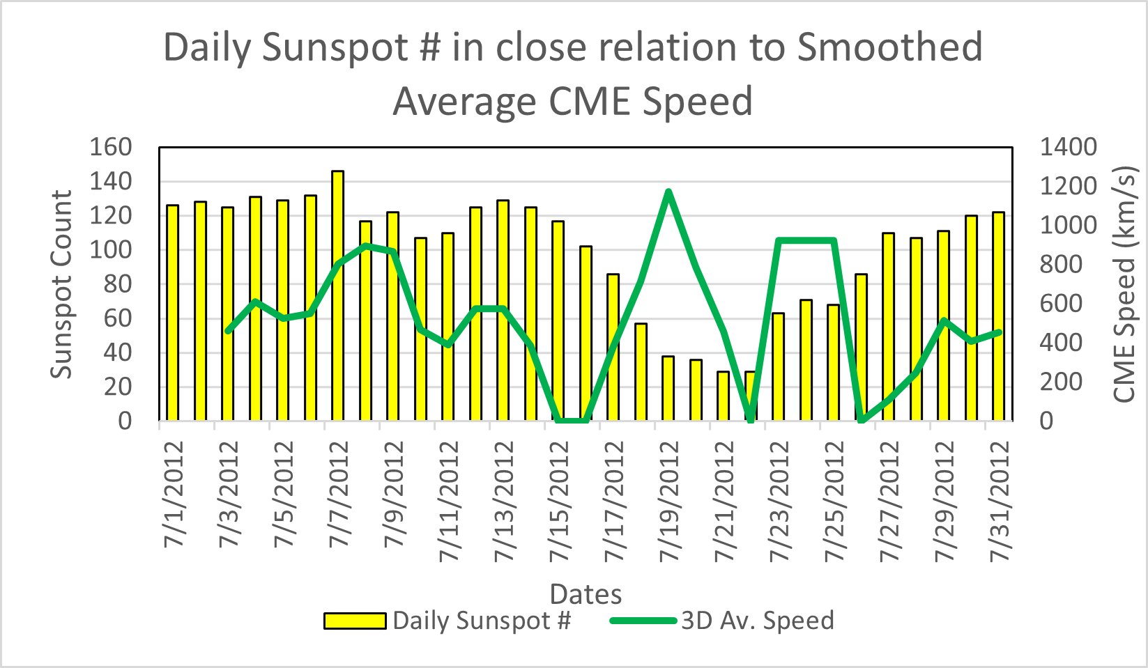
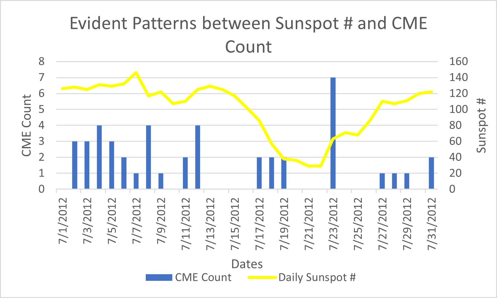
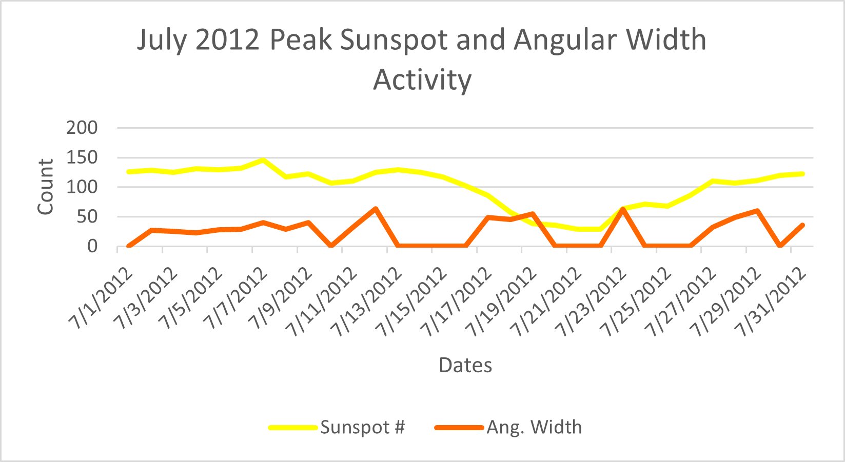
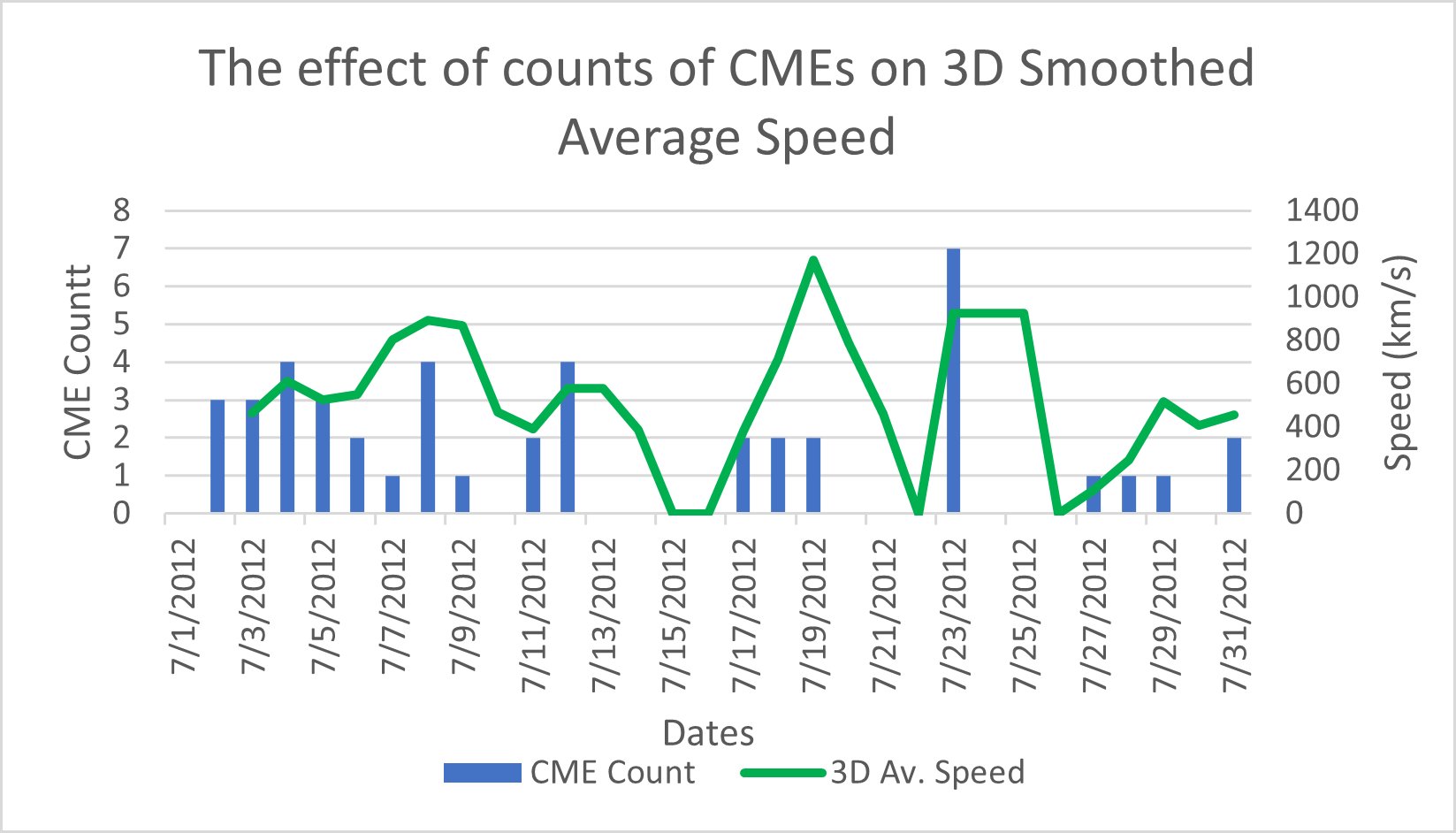
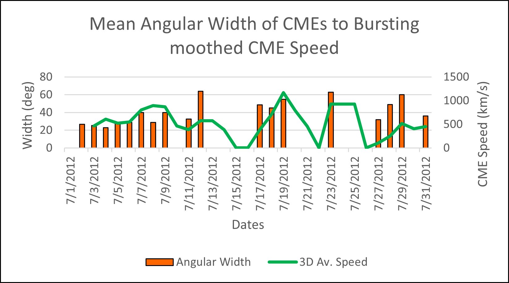The July 2012 burst exhibits elevated burst severity values alongside increased CME frequency. This suggests that high-speed, magnetically intense eruptions are associated with stronger space weather potential. Despite Solar Cycle 24 being relatively weak overall, localized magnetic complexity produced extreme short-term activity.

Evaluating the March 2012 sustained, off-cyclic volatile CME release counteracting the minima nature of Cycle 24.

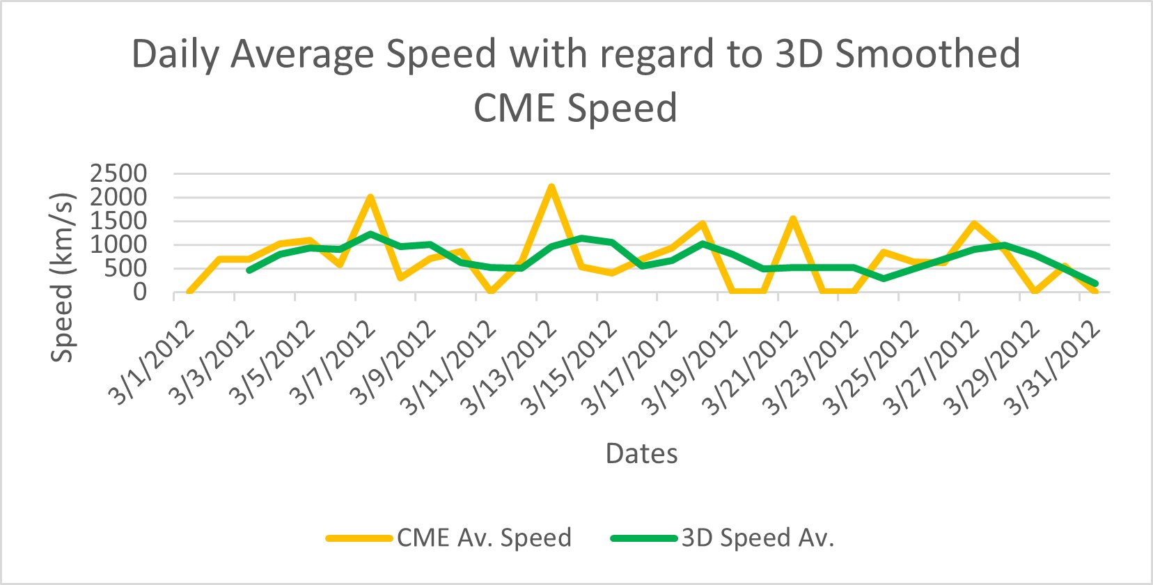
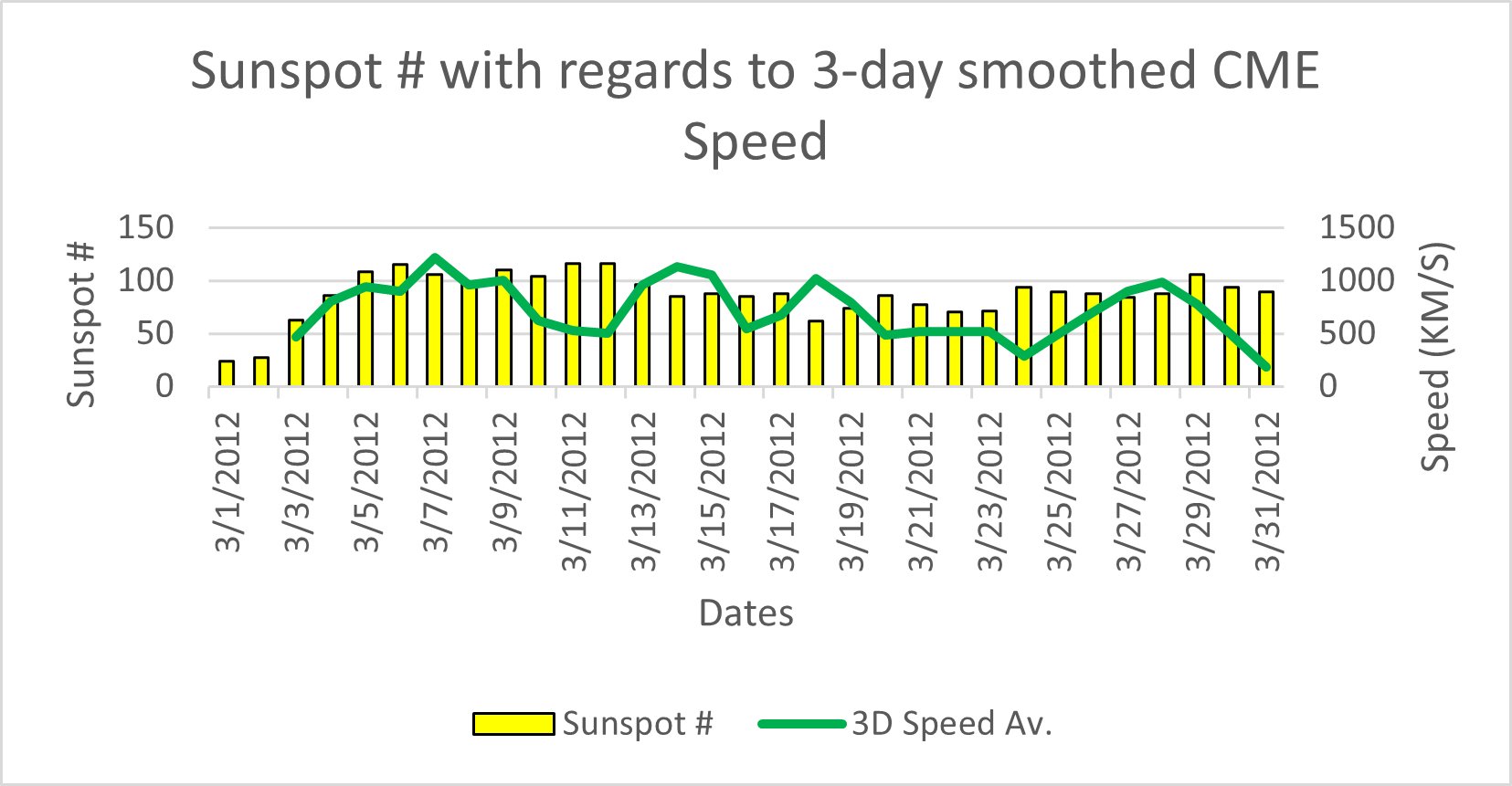
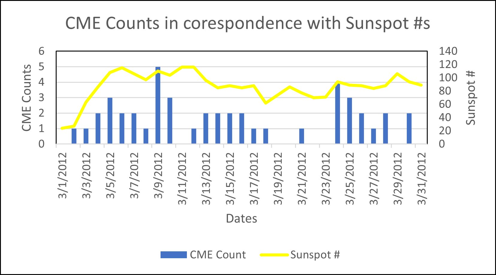
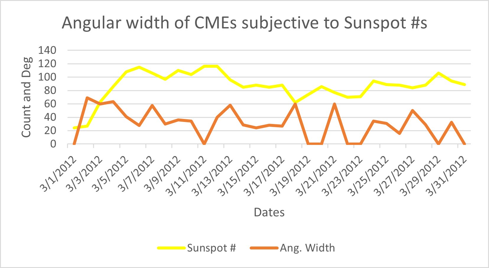
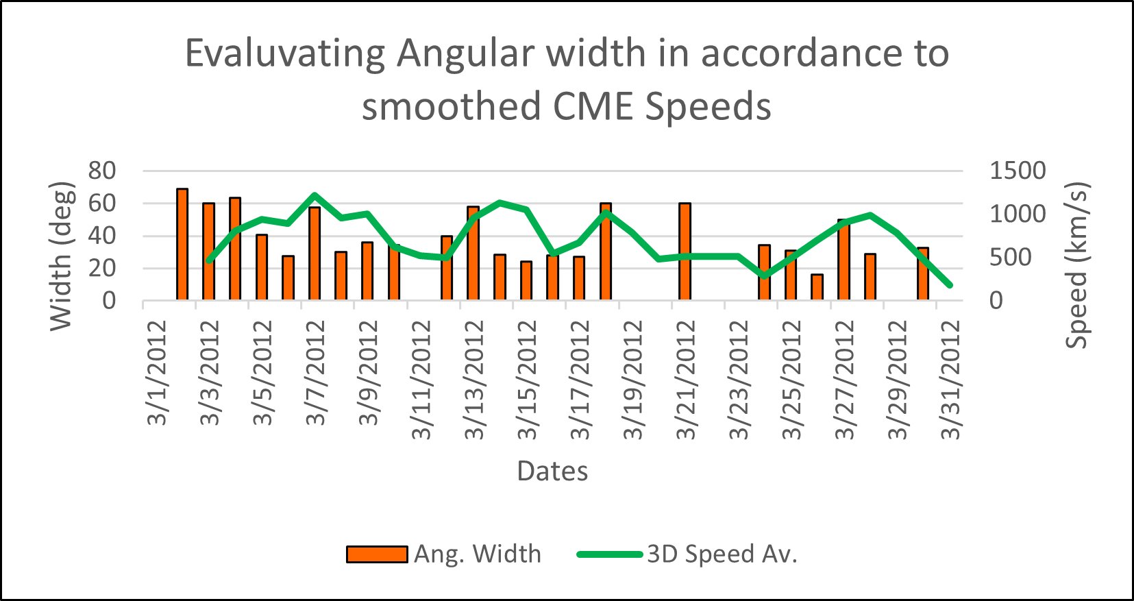The March 2012 burst demonstrates that moderate sunspot levels can still generate high-burst severity, geoeffective CMEs. This highlights the importance of magnetic configuration and directionality, not just total sunspot count, in determining space weather impact.

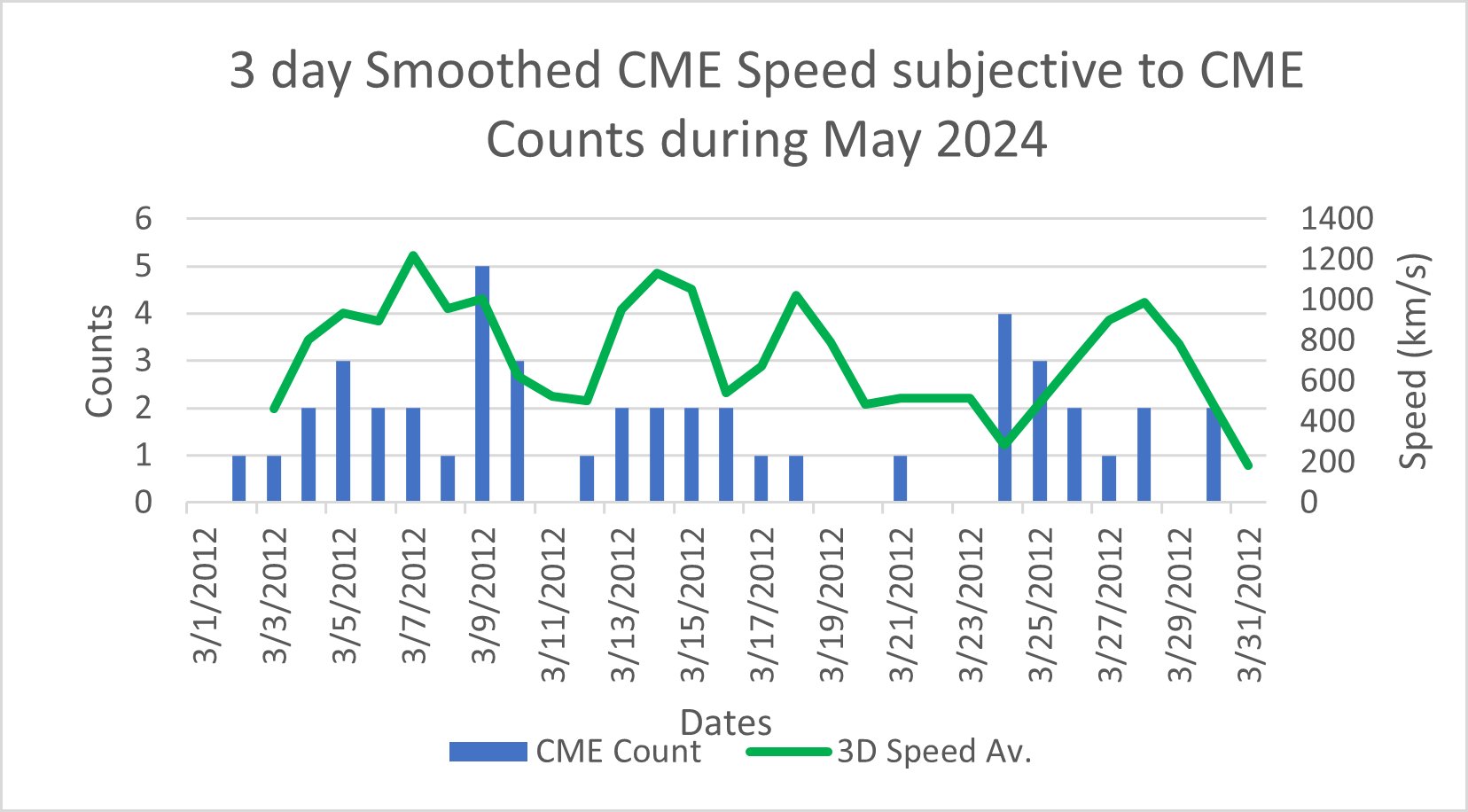
Exploring May 2024 sustained burst severity and high CME volatility

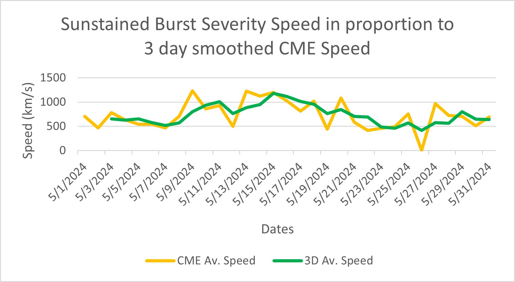
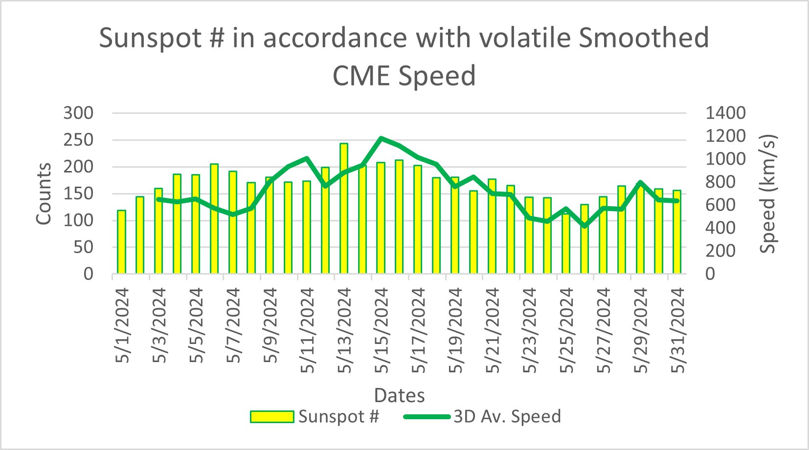
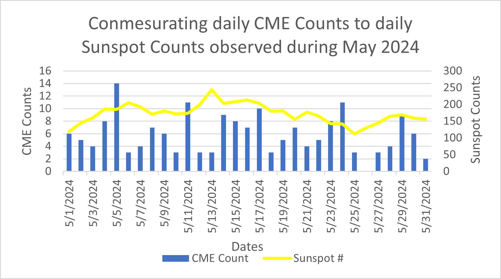
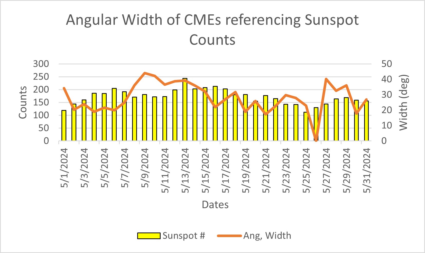
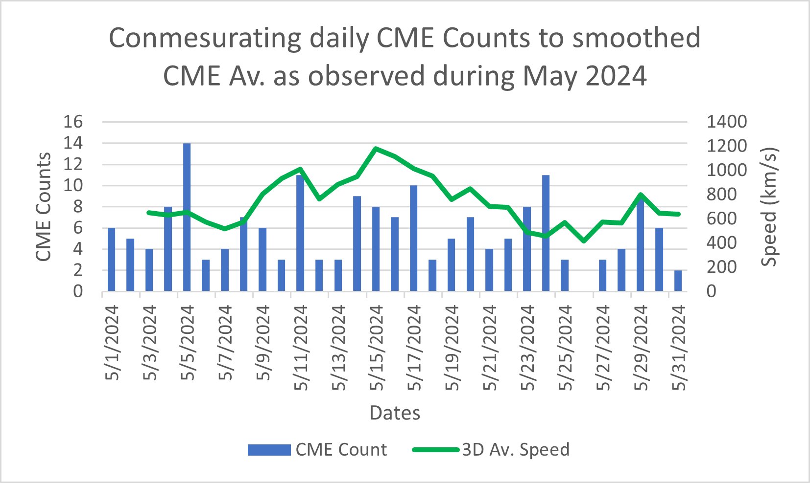
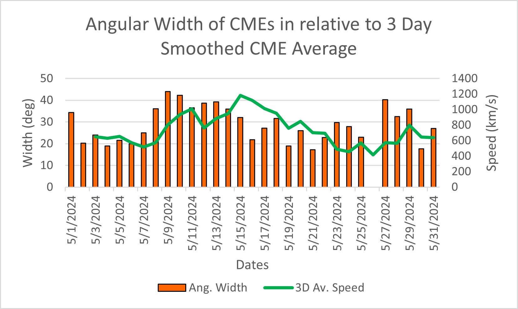The May 2024 burst shows increasing BSI values during the rising phase of Solar Cycle 25. This suggests strengthening magnetic instability in the current cycle and indicates the potential for more intense space weather events as the cycle progresses.  

Comparative Analysis of High Volatility in Cycle 24 and Cycle 2025, highlighting May 2024, Jul 2012 and Mar 2012:

BSI (Burst Severity Index) is a dimensionless index to measure burst severity over multiple time frames developed in this project independently. The equation used for BSI calculations is:

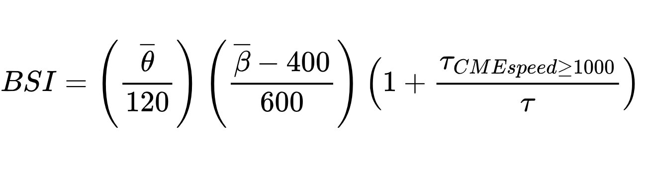
In this equation: β= Mean CME Speed θ = Mean Angular Width τ = Total CME Count Comparing microcycle bursts across Solar Cycles 24 and 25 reveals variation in BSI intensity and CME output. While some bursts show elevated CME frequency with moderate BSI, others exhibit high BSI with fewer total events. This suggests that burst intensity depends not only on event count but also on eruption velocity and magnetic strength.

4.2- Temporal & Spatial Analysis

Temporal analysis revealed scale-dependent behavior between Coronal Mass Ejection (CME) activity and sunspot number, a relationship crucial for understanding solar dynamics. At the macro (solar cycle) level, peak correlation occurred at Lag 0 months, with correlation values ranging from r = 0.85 to 0.99 (pooled r ≈ 0.91), indicating synchronous long-term evolution. Specifically in Solar Cycle 23, the raw correlation number was 0.69 in Lag 0, and a smoothed value of 0.88. Secondly, during Solar Cycle 24, the raw correlation at Lag 0 was 0.86 and a smoothed correlation of 0.98, which is classified an extremely strong correlation during a deep Minima Solar cycle proving that correlation is significant even during periods of passive solar activity. Lastly, Cycle 25 showed a correlation of 0.91 in raw computation and 0.98 when computing a 13-month smoothed average, highlighting the importance of smoothing in revealing underlying trends. This average pooled correlation of 0.91 shows an extremely strong and synchronous correlation between CME occurrences and sunspot correlations highlighted by an average of 82% of all changes being synchronous However, micro-scale analysis of burst events showed peak correlation occurring at short positive lags of approximately 2–5 days. This suggests that localized increases in magnetic complexity, reflected by sunspot formation, precede CME occurrence by several days. CME peaks were observed to cluster near solar maxima while short-term burst activity often followed local sunspot enhancements. Specifically, Nov 2011, Sep 2017, Jul 2012, Mar 2012, and May 2012 had maximum lag values of 1 day, 3 days, 5 days, 1 day, and 1 day respectively. These findings support the interpretation that both phenomena share a common magnetic origin, with CMEs representing a delayed release of stored magnetic energy. Spatial analysis revealed that CME eruptions exhibited significant variation depending on the phase of solar activity. Periods of low activity were associated with narrower and more confined eruptions, while burst intervals with higher BSI values exhibited broader angular widths, indicating larger-scale coronal eruption. Micro off-cycle events such as July 2012 and May 2024 showed rapid spatial expansion of CME structures, consistent with localized magnetic stress release. Across full solar cycles, enhanced CME spatial corresponded with periods of elevated sunspot activity, suggesting that increased magnetic complexity leads to expansive coronal expansion.

5.    Results & Interpretation

5.1 Key Findings

The following key findings summarize correlations, trends, and patterns observed across all sunspot regions, CME occurrences and time periods studied. This analysis highlights five principal findings relevant to understanding solar-cycle behaviour. Firstly, upon analyzing data from Solar Cycles 23, 24 and 25, the Pearson Correlation Coefficient was utilized to calculate correlation. To ensure a robust understanding, both Raw and Smoothed 13 Month average data was calculated independently with the Correlation Coefficient. Upon analyzing the results, the raw graphs had a lower correlation score overall with scores of 0.69, 0.86 and 0.91 with an overall lag of 0 months. On the other hand, the smoothed correlation scores were 0.13 more on average than the raw correlation at a lag of 0. An exception was observed during Solar Cycle 23, when the raw correlation score was the lowest at 0.6888, the smoothed correlation bumped the score up by 0.2 and offset the score by one month, skewing the consistent pattern in all Solar Cycles of being best correlated at lag 0. The data displays that smoothing enhances signal detection in noisier or less correlated periods without significantly distorting timing, making it a reliable method for identifying structured solar-cycle trends. Secondly, examining CME burst volatility clustering and investigating relationships revealed that CME activity does not scale and decline linearly, but instead organize into fleeting bursts of significant ejecta and volatility. These periods of intense solar phenomena are characterized by a dense collection of eruption-prone, high power CME events with extremely unstable phases. The periods that occur right before these eruptive phases are defined as periods with excessive magnetic helicity, decaying coronal arcades and eruptive instabilities. This clustering suggests that extreme solar eruptions are not randomly distributed in time, but instead emerge during concentrated intervals of heightened solar instability. Thirdly, investigation of months falling into intervals of heightened solar eruptions and intense phenomena divulged a temporal relationship in which changes in sunspot observations tend to precede peaks and dips in CME speed. The interval that CME speed follows after sunspot changes varies from 1-5 days, where higher volatility and spikes in these periods of heightened solar activity increases lag compared to a more sustained burst. Juxtaposing the relationship mentioned above is the relationship between the frequency of CMEs and the observations of sunspots. This is because CME frequency has a wild lag range from 3 to -2 which signifies that CME counts and sunspot counts are not related. CME counts and sunspot counts are controlled by different drivers, as CME counts depend more on physical attributes like number of flux ropes and processes of MHD, while sunspots depend more on helicity. This suggests that while sunspots are linked to the presence of CME activity, they are more directly associated with the intensity of eruptions rather than their frequency. Fourthly, cross-validating the data between the full cyclic analysis and micro-burst events disclosed that during the full cyclic analysis, the lag is almost always 0 months except for some cases with extremely altering raw counts. However, upon dissecting some micro-burst phases each lasting one month, the lag varied significantly from 1 day to 5 days. This distinction highlights a scale-dependent temporal behaviour in solar eruptive dynamics. While long-term solar cycles exhibit near-synchronous evolution between sunspot activity and CME occurrences, short-duration burst phases demonstrate measurable delays between surface magnetic activity and eruptive response. These short lags suggest that during intense activity windows, additional physical processes — such as magnetic energy buildup and release — introduce brief but observable timing offsets between sunspot evolution and CME initiation and eruption. Lastly, a comparative analysis of Cycle 24 & 25’s phases with intervals of concentrated bursts of solar activity revealed a great deal about the morphology and structure of both cycles’ points of extreme activity. The two periods taken into account were March 2012 and May 2024, both were possessed an unprecedented number of solar phenomena compared to scientific estimation. Even though Mar 2012 possessed a lot of impulsive spikes of CME speeds reaching a whopping 2000 km/s, the mean of all CME speeds in Mar 2012 was only 689.15 km/s contrasting to the 729.4 km/s observed in May 2024. Even though the mean is higher in May 2024, it still is only a 5.8% increase compared to Mar 2012, which is a barely noticeable change. Hence, 2012 was built with sharp spikes of solar activity while 2024 had a sustained and elevated baseline CME activity. Secondly, upon calculating the Standard Deviation of both cyclic periods, Mar 2012 had a much higher Standard Deviation (speed) of 582 km/s while May 2024 had a Standard deviation of a measly 282.77 km/s, this suggests that May 2024 had a 2x lower Std. Deviation Compared to Mar 2012. Thirdly, upon calculating for the Coefficient of Variation (CV), March 2012 had a CV of 0.84 and May 2024 had a  CV of 0.39 which shows that Mar 2012 had a relative volatility 2x greater than that of May 2024. Cohen’s D between March 2012 and May 2024 was calculated to be approximately 0.0875, indicating a measurable shift in CME speed distributions. Additionally, the Burst Severity Index increased from 0.13356 in March 2012 to 0.16311 in May 2024, representing a \~22% rise in eruptive severity. When compared to the baseline average BSI of 0.0875, March 2012 exhibited a \~53% elevation, while May 2024 showed an \~86% increase. This shows that Cycle 25 had sustained burst periods with limited variability (51 % less than Cycle 24), but a high overall burst severity, but Cycle 24 had more impulsive shocks of high CME activity with magnetic arcades rapidly tangling and reconnecting. Even though some periods in Cycle 24 felt more violent, Cycle 25 usually had more sustained and, thus higher volatility. These finding are as accurate as possible, but are vulnerable to some uncertainties.

5.2 Uncertainty & Error Sources

In this project, all error sources were thought through and optimized such that it does not interfere at all with the main premises and foundation of this project. However, even after significant limitations, some data in this project still remains vulnerable to key issues and data concerns. Firstly, Halo CME percentages were used in our project where we counted the CMEs recorded in a month and divided each by its respective months’ total CME counts. This is not a foolproof method to calculate Halo-based volatility, as it introduces significant mathematical constraints that skew data. For a succinct example, if there is a moderate amount of Halo CMEs which may be 4 and a low number of total CMEs (60) it will skew the average percentage and the percentage will shoot up compared to an average CME count of 125: 4/60 = 1/15 = 6 % compared to 4/125 = 3.2 %     This is about a 2x decrease upon raising the denominator slightly. This demonstrates that percentages can be disproportionately amplified when total counts are low.   This issue persists and is visible in some of my graphs where the raw percentages shoot up to 16% and the smoothed percentages shoot up to 7% which skews data, and highlights a gap of understanding halo-based CME volatility Secondly, some of the data taken in late 2025 for CME counts was taken through secondary, unverified sources out of desperation, with these unauthorized CME counts, the correlation might be skewed for latter part of 2025 and in turn also the Halo-CME numbers may have a slight chance of ending up as flawed. This issue will be coated with less attention paid to past Jul 2025 dates, and their respective averages, however, this data may produce incorrect and inviable information when applied in coding-based prediction systems. Lastly, additional sources of uncertainty include timing resolution and observational consistency. For instance, short-term bursts of activity may be underrepresented due to daily reporting limitations, and some sunspot counts may differ between instruments or catalogs, particularly in SILSO data from the Royal Observatory of Belgium, used extensively for almost all sunspot counts due to easy accessibility and reliable findings. These constraints introduce minuscule variability but do not compromise overall trends or the validity of the main findings. By explicitly acknowledging these limitations, the project provides transparency regarding potential sources of error while maintaining confidence in the broader correlations and interpretations observed, with a small amount of uncertainty during precision points. These findings provide insight into structural complexity and lay the foundation for predictive modelling in Sections 6–7.

6.  Mathematical Modelling

6.1 Key Formulae

To make this project a reality, 11 key formulae had to be used. These formulae varied from statistics calculations, to smoothing proportions to independently developed equations. The processes and usages behind these equations will be described with great detail, and their overall contribution to my project. Firstly, this project had 6 statistics-related equations ranging from elementary to complex-statistics. Statistics was used to compare Cycle 24 & Cycle 25’s overall volatility and to uncover the secrets behind the processes that shape cycles in deep minima and maxima. The first equation used was:

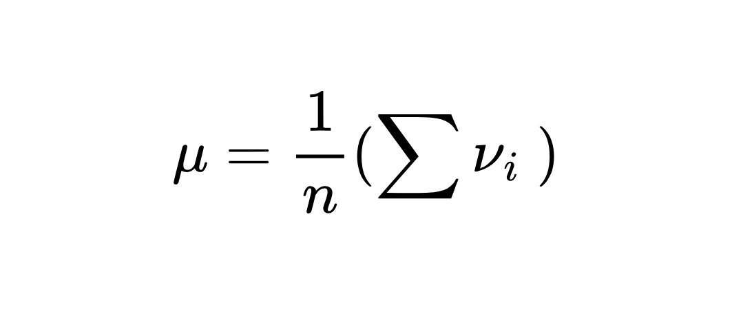
This is the equation for calculating mean of all values in a given dataset, a basic tool used to compare Cycle 24 and 25’s baseline speed. This equation comprises of: ·        μ = average CME speed ·        n = total number of CMEs in that month ·        vᵢ = each individual CME speed ·        Σ (sigma symbol) = “add all of them together” Next is the equation used to calculate the Standard deviation of a given dataset. This equation measures the spread of a dataset and how far are its values from the mean. This was also a basic tool to build the foundation for CME-based micro-cyclic research: This equation comprises of these variables : 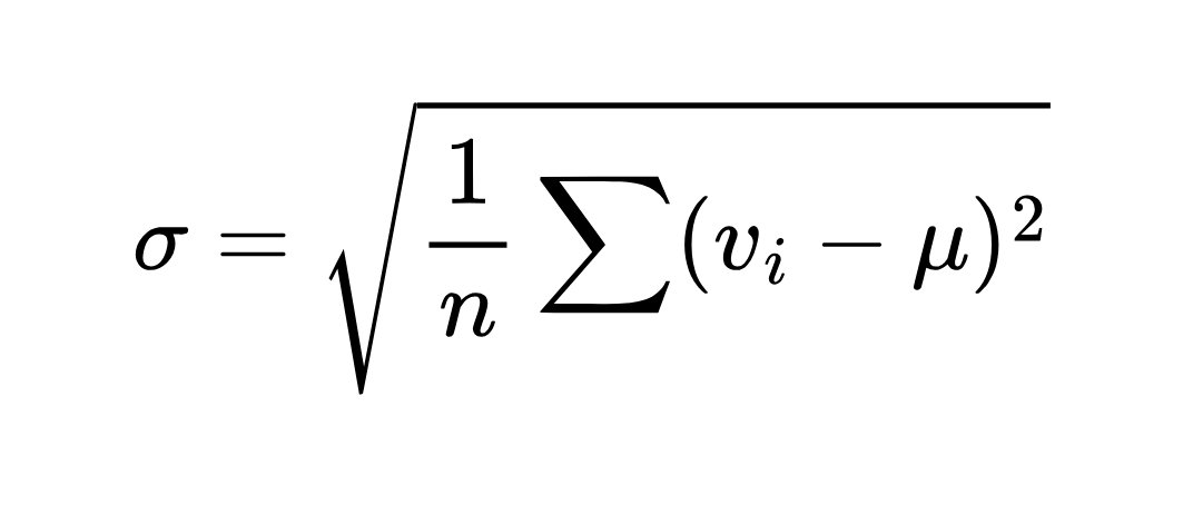·        σ (sigma) = standard deviation ·        vᵢ - μ = how far each CME speed is from the average ·        n = total number of CMEs in that month The third equation used in the statistics calculation is the Coefficient of Variation (CV) which is Volatility divided by the average. This equation was used to tell how large is the spread relative to the mean. For a succinct example, if the CV is over or 0.5, it is significantly high, however it is controlled if it is 0.25 or less. 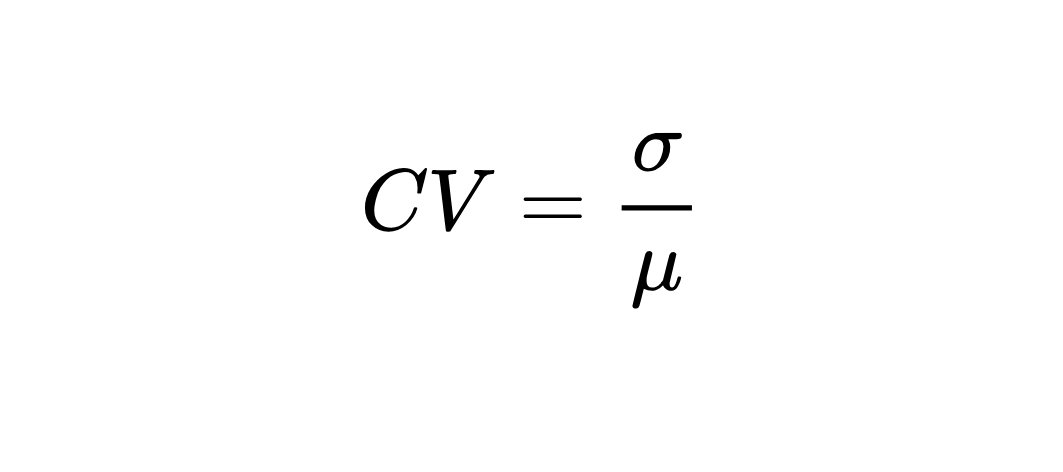·        σ = Standard Derivation (Volatility) ·        μ = Mean of Data (CME Speed)   Fourth in the lineup is the Peak-to-main ratio, which is a ratio that measure the impulsivity of datasets and their values. It is a salient formula that encompasses the peak of the speeds with the mean. 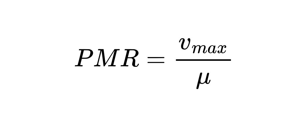This equation consists of these variables: ·        vₘ = fastest CME that month ·        μ = average speed   Fifthly, the statistics formulae contained the formula for a pooled standard derivative which is a combined standard derivative measure that was applied to calculate for Cohen’s D. The formula is as follows:

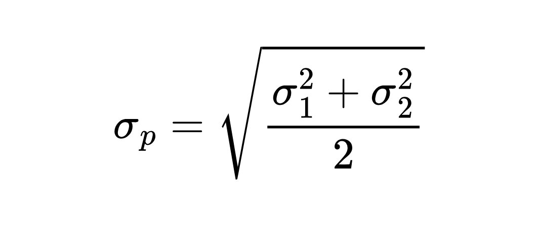
·        s1 = standard deviation of first dataset ·        s2 = standards deviation of second dataset Lastly, in the set of statistics related equations is the Cohen’s D that utilizes the pooled standard deviation shown above. Even though no interesting values came out of the Cohen’s D it is still an integral part of my project. Cohen's D is a standardized effect size measure used to determine the magnitude of the difference between two means, typically in medicinal studies: ·        x = mean of May 2024 ·        μ = mean of March 2012 ·        Sigma = pooled standard deviation Even though the comparison resulted in 0.088 which is quite weak, as the means are very similar, Cohen’s D is an interesting measure, and in our project, displayed how the means are not different significantly but both months are extremely different in Standard deviation and volatility. Next is the formula used for Smoothing in my project, the Gaussian Blurring In 1D formula. This formula is a formula that allows you to smooth the edges, and in turn, removed excess noise from our project’s graphs after heavy smoothing: k = kernel, in short, the value adjustable to match smoothing needs σ=  Standard Deviation. This defines how much weight is given to pixels near the center versus far away, effectively controlling the spread of the Gaussian function. A higher sigma creates a wider, smoother, and more intense blur. While observational heliophysics provides extensive datasets on sunspots and Coronal Mass Ejections (CMEs), raw counts alone often fail to capture the underlying volatility-related complexity of solar eruptive activity. To move beyond descriptive analysis, four independent mathematical indices were developed to quantitatively model structural, temporal, and volatility-based characteristics of solar phenomena. Collectively referred to as the Pratham set, these equations provide a framework for interpreting solar activity through measurable relationships rather than isolated observations. First is the formula most widely used in this project for the analysis of Cycle 24 & Cycle 25 burst months, the BSI or the Burst Severity Index. The Burst Severity Index (BSI) was used to quantify eruptive intensity during burst months. The equation is as follows:

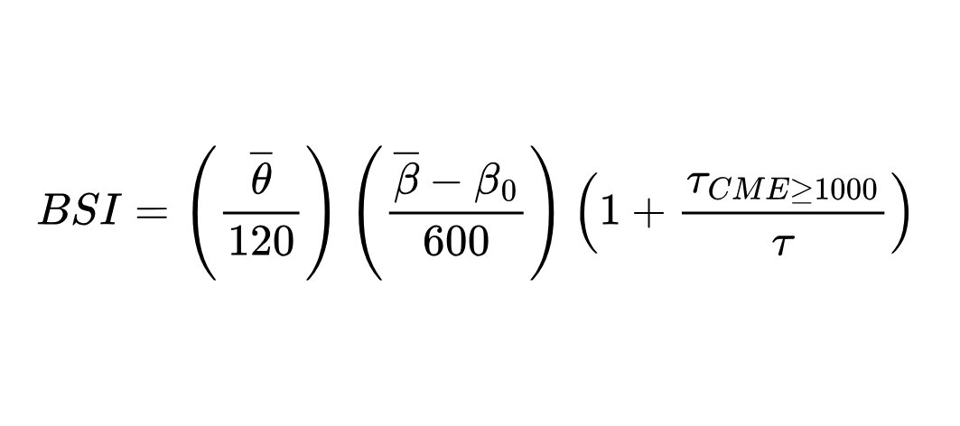
·        Overline θ = Mean Angular Width ·        Overline β = Mean CME Speed ·        τ1000 = Count of CMEs with Speed over 1000km/s ·        τ = Total Count of CMEs ·        I used 120° as that represents a wide CME threshold. ·        I utilized 400 km/s because it is near the average solar wind speed. ·        I made use of 600 km/s because it scales typical CME variation This equation was independently developed while exploring the data of this project to make up for the lack of unifying CME severity indices. To make the BSI dimension less, I grouped similar measures with each other and divided them by each other to cancel out terms and make a level, dimensionless index. Second is the SEP, or the Sunspot Eruptive Probability is another measure that encompasses all aspects of a possibility of local eruption including eruptions that originate from the magnetic helicity that formed the Sunspots.

• σ (sigma) — gas pressure in the sunspot region
• γ (gamma) — magnetic influence
• d — sunspot diameter
• v — surface area of the sunspot
• — average surface area of sunspots (≈ 289,000,000 km²)
• Vmax — maximum observed surface area
• τ δ — number of delta-class sunspots in the region
• τ — total sunspot counts in the region
• g — number of previously eruptive sunspots

This formula normalizes each parameter relative to average values to quantify deviations from typical solar behaviour. The multiplicative structure captures interactions among thermodynamic, magnetic, geometric, and historical variables, while the additive term incorporates prior eruptive activity. Higher values of this complexity index indicate regions that are structurally more intricate and potentially more likely to produce significant solar events. By integrating multiple factors, this model provides a quantitative tool to assess sunspot complexity in a standardized and interpretable manner. Another Independent formula to rank Sunspot Group Erupt ability is as follows:

• fi, f1 — angular positions of sunspot features represented on a unit circle, with the side facing Earth corresponding to radians and the side facing away corresponding to radians. Differences between these angles ( ) capture spatial orientation and relative positioning of sunspot regions.
• l — linear displacement factor of the sunspot region
• Δ — change in activity relative to previous observations
• A — sunspot area
• S — sunspot complexity score (e.g., from the previous complexity formula)
• K1, K2 K3— scaling coefficients to weight the contributions of activity change, area, and complexity

The sine component of the formula reflects the relative orientation of sunspots in heliographic coordinates, with higher values indicating greater angular separation relevant to Earth-facing activity. The additive terms incorporate physical and activity-based parameters, producing a composite metric for each region. Higher SGE values correspond to more dynamic or geometrically significant sunspot events, allowing the formula to complement the previously defined complexity index and provide a multi-dimensional perspective on solar activity.   A further original formula, denoted HRS, was developed to integrate magnetic, temporal, and geometric factors in evaluating solar activity:

where the variables are defined as follows:

• — southward magnetic field component of the sunspot region
• — reference magnetic field value for normalization
• Δr — change in CME count between the previous month and the current month
• Δs — change in Halo CME percentage between the previous month and the current month
• l — linear displacement of the sunspot region
• — reference linear displacement for normalization
• ,  — angular positions of sunspot features on a unit circle, capturing spatial orientation and Earth-facing geometry

The formula combines magnetic intensity, temporal changes in CMEs and Halo CMEs, linear displacement, and angular positioning to produce a composite metric reflecting solar activity dynamics. The weighted sum of magnetic strength and changes in CME and Halo counts captures evolving solar conditions, while the geometric term reflects the relative orientation of features in heliographic coordinates. In practice, situations may arise where the change in Halo CMEs exceeds the change in total CME counts; however, this does not pose a computational issue for the formula, as the absolute value ensures meaningful contributions from both terms. Higher HRS values correspond to regions of increased magnetic activity and evolving CME dynamics, complementing other indices such as SGE and the complexity index to provide a comprehensive multi-factor assessment of solar regions.

CITATION & REFERNCES

In Harvard-Style Citations

1. Schwenn, R., Dal Lago, A., Huttunen, E. and Gonzalez, W.D., 2005, March. The association of coronal mass ejections with their effects near the Earth. In Annales geophysicae (Vol. 23, No. 3, pp. 1033-1059). Göttingen, Germany: Copernicus Publications.

2.      NOAA (2019). Coronal Mass Ejections | NOAA / NWS Space Weather Prediction Center. [online] Noaa.gov. Available at: https://www.swpc.noaa.gov/phenomena/coronal-mass-ejections. 3.      ‌NOAA (n.d.). NOAA Space Weather Scales | NOAA / NWS Space Weather Prediction Center. [online] www.swpc.noaa.gov. Available at: https://www.swpc.noaa.gov/noaa-scales-explanation. 4.      Wikipedia Contributors (2019). Coronal mass ejection. [online] Wikipedia. Available at: https://en.wikipedia.org/wiki/Coronal_mass_ejection. 5.      Klein, C. (2012). A Perfect Solar Superstorm: The 1859 Carrington Event | HISTORY. [online] HISTORY. Available at: https://www.history.com/articles/a-perfect-solar-superstorm-the-1859-carrington-event. 6.      Wordcounter.net. (2013). Character Counter - WordCounter.net. [online] Available at: https://wordcounter.net/character-count. 7.      NASA (n.d.). Sun: Exploration - NASA Science. [online] science.nasa.gov. Available at: https://science.nasa.gov/sun/exploration/. 8.      Wikipedia. (2022). Solar maximum. [online] Available at: https://en.wikipedia.org/wiki/Solar_maximum. 9.      NASA (n.d.). Space Technology 5. [online] www.jpl.nasa.gov. Available at: https://www.jpl.nasa.gov/nmp/st5/SCIENCE/cme.html. 10.    Y.;Luhmann, L. (2011). CME Flux ropes: Origins, Characteristics and Consequences. AGU Fall Meeting Abstracts, [online] 2011, pp.SH42A03. Available at: https://ui.adsabs.harvard.edu/abs/2011AGUFMSH42A..03L/abstract [Accessed 8 Jan. 2026]. 11.     Eleni (2024). Properties of Magnetic Polarity Inversion Lines Revealed by DKIST ViSP Observations. AGU Fall Meeting Abstracts, [online] 2024(2914), pp.SH21G2914. Available at: https://ui.adsabs.harvard.edu/abs/2024AGUFMSH21G2914B/abstract [Accessed 8 Jan. 2026]. 12.     MyBib Contributors (2019). Harvard Referencing Generator – FREE – (updated for 2019). [online] MyBib. Available at: https://www.mybib.com/tools/harvard-referencing-generator. 13.     Nindos, A., Zhang, J. and Zhang, H. (2003). The Magnetic Helicity Budget of Solar Active Regions and Coronal Mass Ejections. The Astrophysical Journal, 594(2), pp.1033–1048. doi:https://doi.org/10.1086/377126. 14.    Government of Canada, N.R.C. (n.d.). Learning about space weather. [online] www.spaceweather.gc.ca. Available at: https://www.spaceweather.gc.ca/info-gen/index-en.php. 15.    Google (2024). ‎Gemini. [online] gemini.google.com. Available at: https://gemini.google.com. 16.     Gopalswamy, N. and M, D.J. (2010). Coronal Mass Ejections: a Summary of Recent Results. [online] Nasa.gov. Available at: https://ntrs.nasa.gov/citations/20100030618 [Accessed 11 Jan. 2026]. 17.     Physics Frontier (2025). What Are The Different Types Of Coronal Mass Ejections? - Physics Frontier. [online] YouTube. Available at: https://www.youtube.com/watch?v=eFzAG05mcaM [Accessed 11 Jan. 2026]. 18.    SpaceWeatherLive.com. (2024). The magnetic classification of sunspots | Help. [online] Available at: https://www.spaceweatherlive.com/en/help/the-magnetic-classification-of-sunspots.html. 19.     Chen, P.F. (2011). Coronal Mass Ejections: Models and Their Observational Basis. Living Reviews in Solar Physics, 8. doi:https://doi.org/10.12942/lrsp-2011-1. 20.    Florido-Llinas, M., Nieves-Chinchilla, T. and Linton, M.G. (2020). Analysis of the Helical Kink Stability of Differently Twisted Magnetic Flux Ropes. 295(9). doi:https://doi.org/10.1007/s11207-020-01687-z. 21.     Chen, Y., Hu, Y.Q. and Xia, L.D. (2007). Two energy release processes for CMEs: MHD catastrophe and magnetic reconnection. Advances in Space Research, [online] 40(12), pp.1780–1786. doi:https://doi.org/10.1016/j.asr.2007.02.011. 22.    Wikipedia Contributors (2024). Quadrupole. [online] Wikipedia. Available at: https://en.wikipedia.org/wiki/Quadrupole. 23.    OpenAI (2025). ChatGPT. [online] chatgpt.com. Available at: https://chatgpt.com. 24.    Wikipedia Contributors (2019). Quasistatic process. [online] Wikipedia. Available at: https://en.wikipedia.org/wiki/Quasistatic_process 25.    NASA (2024). Sunspots - NASA Science. [online] Nasa.gov. Available at: https://science.nasa.gov/sun/sunspots/. 26.    ielts.idp.com. (n.d.). Grammar 101 | Affect vs Effect: Learn the difference | IDP IELTS. [online] Available at: https://ielts.idp.com/canada/prepare/article-grammar-101-affect-vs-effect. 27.    Wikipedia Contributors (2025). Sunspot. Wikipedia. 28.    CalculatorSoup, L. (2019). Temperature Conversion Calculator. [online] CalculatorSoup. Available at: https://www.calculatorsoup.com/calculators/conversions/temperature.php. 29.    Solanki, S.K. (2003). Sunspots: An overview. Astronomy and Astrophysics Review, 11(2-3), pp.153–286. doi:https://doi.org/10.1007/s00159-003-0018-4. 30.    Dobrijevic, D. (2022). Sunspots: What are they, and why do they occur? [online] Space.com. Available at: https://www.space.com/sunspots-formation-discovery-observations. 31.     www.unitconverters.net. (n.d.). Convert Tesla to Gauss. [online] Available at: https://www.unitconverters.net/magnetic-flux-density/tesla-to-gauss.htm. 32.    Mathda.com. (2026). Tesla to Microtesla converter (T to µT) - MathDA.com. [online] Available at: https://mathda.com/convert/magneticfield/tesla-to-micro-tesla [Accessed 25 Jan. 2026]. 33.    soho.nascom.nasa.gov. (n.d.). How Are Magnetic Fields Related To Sunspots? [online] Available at: https://soho.nascom.nasa.gov/explore/lessons/sunspots6_8.html. 34.   NSF - National Science Foundation. (2011). How the Sun Gets Its Spots. [online] Available at: https://www.nsf.gov/news/how-sun-gets-its-spots. 35.    Birx, H. (2009). Encyclopedia of Time: Science, Philosophy, Theology, & Culture. doi:https://doi.org/10.4135/9781412963961. 36.    Archive.org. (2026). Spaceflight Now | Breaking News | SOHO reveals how sunspots take stranglehold on the Sun. [online] Available at: https://web.archive.org/web/20150117214759/http://www.spaceflightnow.com/news/n0111/06sunspots/ [Accessed 25 Jan. 2026]. 37.    Chapter 3. (2003). Available at: https://www.ngdc.noaa.gov/stp/space-weather/solar-data/solar-features/sunspot-regions/usaf_mwl/documentation/usaf_sunspot-analysis-techniques_afwaman15-1.pdf. 38.    SpaceWeatherLive.com. (2024). The magnetic classification of sunspots | Help. [online] Available at: https://www.spaceweatherlive.com/en/help/the-magnetic-classification-of-sunspots.html. 39.    American Association for the Advancement of Science (AAAS). (2026). Science: Pinpointing the Nature of Filaments in Sunspots | American Association for the Advancement of Science (AAAS). [online] Available at: https://www.aaas.org/news/science-pinpointing-nature-filaments-sunspots [Accessed 26 Jan. 2026]. 40.   Cysf.org. (2024). CYSF. [online] Available at: https://platform.cysf.org/project/browse/. 41.    Chapter 3. (2003). Available at: https://www.ngdc.noaa.gov/stp/space-weather/solar-data/solar-features/sunspot-regions/usaf_mwl/documentation/usaf_sunspot-analysis-techniques_afwaman15-1.pdf. (Note: For Writing 2.5 Key Terminologies) 42.    https://www.howstuffworks.com/about-patrick-j-kiger.htm (2009). How Sunspots Work. [online] HowStuffWorks. Available at: https://science.howstuffworks.com/sunspot3.htm. 43.   Encyclopedia Britannica. (n.d.). Sunspot | astronomy. [online] Available at: https://www.britannica.com/science/sunspot. 44.   Allen, J., Sauer, H., Frank, L. and Reiff, P. (1989). Effects of the March 1989 solar activity. Eos, Transactions American Geophysical Union, 70(46), p.1479. doi:https://doi.org/10.1029/89eo00409. 45.   Irie, (2026). Large sunspot group of March 1989 (NOAA 5395). Report of the National Astronomical Observatory of Japan, [online] 1(2), pp.193–211. Available at: https://ui.adsabs.harvard.edu/abs/1991RNAOJ...1..193I/abstract [Accessed 30 Jan. 2026]. 46.    Phillips, D.T. (2021). The Great Québec Blackout. [online] Spaceweather.com. Available at: https://spaceweatherarchive.com/2021/03/12/the-great-quebec-blackout/. 47.    Wikipedia. (2021). July 2012 solar storm. [online] Available at: https://en.wikipedia.org/wiki/July_2012_solar_storm. 48.   science.nasa.gov. (2014). Near Miss: The Solar Superstorm of July 2012 - NASA Science. [online] Available at: https://science.nasa.gov/science-research/planetary-science/23jul_superstorm/. 49.    ScienceDaily. (2026). Fierce 2012 magnetic storm just missed us: Earth dodged huge magnetic bullet from the sun. [online] Available at: https://www.sciencedaily.com/releases/2014/03/140318154940.htm [Accessed 30 Jan. 2026]. 50.   ESA (2025). ESA analyses impacts of November 2025 solar storm after three CMEs strike Earth. [online] aerospace-and-defence. Available at: https://www.aerospace-and-defence.com/esa-analyses-impacts-november-2025-solar-storm-3-cmes-earth-a-2234835b9110a63fc0c49764ea83ecbd/?utm_source=chatgpt.com [Accessed 30 Jan. 2026]. 51.    Buckle, A. and Hocken, V. (2019). UTC – Coordinated Universal Time. [online] Timeanddate.com. Available at: https://www.timeanddate.com/time/aboututc.html. 52.    Baker, H. (2026). Earth hit by biggest ‘solar radiation storm’ in 23 years, triggering Northern Lights as far as Southern California. [online] Live Science. Available at: https://www.livescience.com/space/the-sun/earth-hit-by-biggest-solar-radiation-storm-in-23-years-triggering-northern-lights-as-far-as-southern-california. 53.    Dobrijevic, D. (2026). Sun unleashes powerful X-flare, CME hits Earth sparking severe geomagnetic storm. [online] Space. Available at: https://www.space.com/astronomy/sun/sun-erupts-with-powerful-x-class-flare-as-huge-cme-races-toward-earth-impact-possible-within-24-hours. 54.   www.spaceweatherlive.com. (n.d.). StackPath. [online] Available at: https://www.spaceweatherlive.com/en/solar-activity/solar-flares.html. 55.    Westernfinancialgroup.ca. (2025). What are solar flares? [online] Available at: https://westernfinancialgroup.ca/What-is-the-Impact-of-Solar-Flares [Accessed 30 Jan. 2026]. 56.    National Oceanic and Atmospheric Administration (n.d.). Solar Flares (Radio Blackouts) | NOAA / NWS Space Weather Prediction Center. [online] www.swpc.noaa.gov. Available at: https://www.swpc.noaa.gov/phenomena/solar-flares-radio-blackouts.‌ 57.    Shukla, P. (2026). Ionization: Explained Simply. [offline] Chemistry 101p. Available at: https://ionization%20in%20simple%20terms. [Accessed 30 Jan. 2026]. Ionization. (My Mother)(Not real Website) 58.   Elvidge, S. and Angling, M.J. (2018). Using Extreme Value Theory for Determining the Probability of Carrington-Like Solar Flares. Space Weather, 16(4), pp.417–421. doi:https://doi.org/10.1002/2017sw001727. 59.    Connors, M. (2024). Sunspots and solar flares, created by the sun’s magnetism, can affect the Earth’s surface. [online] The Conversation. Available at: https://theconversation.com/sunspots-and-solar-flares-created-by-the-suns-magnetism-can-affect-the-earths-surface-230208. 60.    Encyclopedia Britannica. (n.d.). Ionosphere and magnetosphere | atmospheric science. [online] Available at: https://www.britannica.com/science/ionosphere-and-magnetosphere 61.     This vs. That. (2023). Coronal Mass Ejection vs. Solar Flare - What’s the Difference? | This vs. That. [online] Available at: https://thisvsthat.io/coronal-mass-ejection-vs-solar-flare?utm_source=chatgpt.com [Accessed 31 Jan. 2026]. 62.    NASA (2018). What is a Lagrange Point? - NASA Science. [online] science.nasa.gov. Available at: https://science.nasa.gov/resource/what-is-a-lagrange-point/. 63.    NESDIS (n.d.). DSCOVR: Deep Space Climate Observatory. [online] NESDIS. Available at: https://www.nesdis.noaa.gov/current-satellite-missions/currently-flying/dscovr-deep-space-climate-observatory. 64.    NASA (n.d.). Sun: Exploration - NASA Science. [online] science.nasa.gov. Available at: https://science.nasa.gov/sun/exploration/. 65.    Noaa.gov. (2019). Real Time Solar Wind | NOAA / NWS Space Weather Prediction Center. [online] Available at: https://www.swpc.noaa.gov/products/real-time-solar-wind 66.     Dobrijevic, D. (2025). ‘We must replace this capability now’: New NOAA satellite to replace aging space weather sentinels launches Sept. 23. [online] Space. Available at: https://www.space.com/space-exploration/satellites/we-must-replace-this-capability-now-new-noaa-satellite-to-replace-aging-space-weather-sentinels-launches-sept-23. 67.    NASA (n.d.). DSCOVR - NASA Science. [online] science.nasa.gov. Available at: https://science.nasa.gov/mission/dscovr/. 68.    NASA (n.d.). ACE - NASA Science. [online] science.nasa.gov. Available at: https://science.nasa.gov/mission/ace/. 69.    ESA (n.d.). SOHO overview. [online] www.esa.int. Available at: https://www.esa.int/Science_Exploration/Space_Science/SOHO_overview2. 70.    SOHO. (2019). Launch Information - SOHO - Science Portal. [online] Available at: https://sci.esa.int/web/soho/-/33613-launch-information [Accessed 1 Feb. 2026]. 71.     NASA (n.d.). SOHO - NASA Science. [online] science.nasa.gov. Available at: https://science.nasa.gov/mission/soho/. 72.    NASA (2014). A First for NASA’s IRIS: Observing a Gigantic Eruption of Solar Material. [online] NASA Scientific Visualization Studio. Available at: https://svs.gsfc.nasa.gov/11556/ [Accessed 1 Feb. 2026]. 73.    Wikipedia Contributors (2025). Interface Region Imaging Spectrograph. Wikipedia. 74.    Interface Region Imaging Spectrograph (IRIS): Understanding how the sun powers its million-degree atmosphere. (2013). Available at: https://www.nasa.gov/wp-content/uploads/2015/03/754247main_iris_press_kit.pdf?emrc=4470f9 [Accessed 1 Feb. 2026]. 75.    Harvard.edu. (2025). Interface Region Imaging Spectrograph (IRIS) | Center for Astrophysics | Harvard & Smithsonian. [online] Available at: https://www.cfa.harvard.edu/facilities-technology/telescopes-instruments/interface-region-imaging-spectrograph-iris. 76.    Nandy, D., Baruah, Y., Bhowmik, P., Dash, S., Gupta, S., Hazra, S., Lekshmi, B., Pal, S., Pal, S., Roy, S., Saha, C. and Sinha, S. (2023). Causality in heliophysics: Magnetic fields as a bridge between the Sun’s interior and the Earth’s space environment. Journal of Atmospheric and Solar-Terrestrial Physics, [online] 248, p.106081. doi:https://doi.org/10.1016/j.jastp.2023.106081. 77.    www.esa.int. (2020). Types of orbits. [online] Available at: https://www.esa.int/Enabling_Support/Space_Transportation/Types_of_orbits#GEO. 78.    sdo.gsfc.nasa.gov. (n.d.). SDO | Solar Dynamics Observatory. [online] Available at: https://sdo.gsfc.nasa.gov/data/. 79.    July 2018, E.H. 13 (n.d.). Solar Dynamics Observatory: Staring at the Sun. [online] Space.com. Available at: https://www.space.com/22081-solar-dynamics-observatory.html. 80.   Pesnell, W.D., Thompson, B.J. and Chamberlin, P.C. (2011). The Solar Dynamics Observatory (SDO). Solar Physics, [online] 275(1-2), pp.3–15. doi:https://doi.org/10.1007/s11207-011-9841-3. 81.    NASA (2023). SDO. [online] NASA Science. Available at: https://science.nasa.gov/mission/sdo/. 82.    Laboratory for Atmospheric and Space Physics. (2022). SDO. [online] Available at: https://lasp.colorado.edu/missions/sdo/. 83.    Nashiket Premlal Parate, Nigar Shaji, Srikanth, M., K. Sankarasubramanian, Patnaik, N.M., S. Narendra, Abhijit Avinash Adoni, Negi, K., Pragyan Pattanaik, Bharat, Subramanian, V.R., Kumar, H., Sahu, S.N., Pai, V.K., Mustafa, S.F., Pathak, R., Amit Maji, Haridas, T.R., Raj, A. and Agarwal, P. (2025). Aditya-L1 - An Observatory Class Mission: Spacecraft, Mission, and Operations. Solar Physics, [online] 300(9). doi:https://doi.org/10.1007/s11207-025-02533-w. 84.   www.isro.gov.in. (n.d.). ADITYA-L1. [online] Available at: https://www.isro.gov.in/Aditya_L1.html. 85.   Historic First: India’s Solar Ultra-violet Imaging Telescope (SUIT) onboard Aditya-L1 Captures Unprecedented Solar Flare Details. (2025). Isro.gov.in. [online] doi:https://doi.org/10.3847/2041-8213/adb0be%3C. 86.    Gbmb.org. (2026). Gbit to GB Conversion Gigabits to Gigabytes Calculator. [online] Available at: https://www.gbmb.org/gbit-to-gb [Accessed 3 Feb. 2026]. 87.    Isro.gov.in. (2023). Aditya-L1 has commenced the collection of scientific data. [online] Available at: https://www.isro.gov.in/Aditya_L1_collection_of_scientific_data.html [Accessed 2 Feb. 2026]. 88.   NASA. (2020). Solar Orbiter Launch Takes Solar Science to New Heights - NASA. [online] Available at: https://www.nasa.gov/news-release/solar-orbiter-launch-takes-solar-science-to-new-heights/ [Accessed 2 Feb. 2026]. 89.    www.esa.int. (n.d.). Launching and operating Solar Orbiter. [online] Available at: https://www.esa.int/Science_Exploration/Space_Science/Solar_Orbiter/Launching_and_operating_Solar_Orbiter. 90.    www.esa.int. (n.d.). Solar Orbiter. [online] Available at: https://www.esa.int/Science_Exploration/Space_Science/Solar_Orbiter. 91.     www.esa.int. (n.d.). Solar Orbiter discovers tiny jets that could power the solar wind. [online] Available at: https://www.esa.int/Science_Exploration/Space_Science/Solar_Orbiter/Solar_Orbiter_discovers_tiny_jets_that_could_power_the_solar_wind. 92.    EurekAlert! (2025). Unlocking the secrets of the Sun’s poles. [online] Available at: https://www.eurekalert.org/news-releases/1099725 [Accessed 3 Feb. 2026]. 93.    science.nasa.gov. (n.d.). STEREO A & B - NASA Science. [online] Available at: https://science.nasa.gov/mission/stereo/. 94.    Wikipedia Contributors (2025). STEREO. Wikipedia. 95.    Nasa.gov. (2024). STEREO. [online] Available at: https://stereo.gsfc.nasa.gov/spacecraft.shtml. 96.    NASA. (2016). NASA Establishes Contact With STEREO Mission - NASA. [online] Available at: https://www.nasa.gov/directorates/somd/space-communications-navigation-program/nasa-establishes-contact-with-stereo-mission/ [Accessed 3 Feb. 2026]. 97.    Wikipedia. (2023). Aditya-L1. [online] Available at: https://en.wikipedia.org/wiki/Aditya-L1. 98.    Nasa.gov. (2025). STEREO - Science Center - Where is STEREO? [online] Available at: https://stereo-ssc.nascom.nasa.gov/where.shtml. 99.    Tavares, M. (2011). Influence of Solar Cycles on Earthquakes. AGU Fall Meeting Abstracts, [online] 2011, pp.NH33A1552. Available at: https://ui.adsabs.harvard.edu/abs/2011AGUFMNH33A1552T/abstract [Accessed 8 Feb. 2026]. 100.  Silverman, S.M. and Hayakawa, H. (2021). The Dalton Minimum and John Dalton’s Auroral Observations. Journal of Space Weather and Space Climate, 11, p.17. doi:https://doi.org/10.1051/swsc/2020082. 101.   Emerson, R.M., Saha, N., Burli, P.H., Klinger, J.L., Bhattacharjee, T. and Vega-Montoto, L. (2024). Analyzing Potential Failures and Effects in a Pilot-Scale Biomass Preprocessing Facility for Improved Reliability. Energies, [online] 17(11), pp.2516–2516. doi:https://doi.org/10.3390/en17112516. 102.  Interrante, A. (2025). NASA’s PUNCH Mission to Revolutionize Our View of Solar Wind. [online] NASA Science. Available at: https://science.nasa.gov/science-research/heliophysics/nasas-punch-mission-to-revolutionize-view-of-solar-wind/. 103.  Noaa.gov. (2025). Coronagraph | NOAA / NWS Space Weather Prediction Center. [online] Available at: https://www.swpc.noaa.gov/products/coronagraph. 104.  Wikipedia Contributors (2019). Maunder Minimum. [online] Wikipedia. Available at: https://en.wikipedia.org/wiki/Maunder_Minimum. 105.  Buckle, A. and Hocken, V. (2019). UTC – Coordinated Universal Time. [online] Timeanddate.com. Available at: https://www.timeanddate.com/time/aboututc.html. 106.  Evans, R.M., Pulkkinen, A.A., Zheng, Y., Leila Mays, M., Taktakishvili, A., Kuznetsova, M.M. and Hesse, M. (2013). The SCORE Scale: A Coronal Mass Ejection Typification System Based On Speed. Space Weather, 11(6), pp.333–334. doi:https://doi.org/10.1002/swe.20058. 107.  Quillbot (2024). AI Detector - QuillBot AI. [online] Quillbot.com. Available at: https://quillbot.com/ai-content-detector. 108.  Wikipedia. (2021). Solar core. [online] Available at: https://en.wikipedia.org/wiki/Solar_core. 109.  Interrante, A. (2023). Layers of the Sun. [online] NASA Science. Available at: https://science.nasa.gov/blogs/the-sun-spot/2023/09/26/layers-of-the-sun/. 110.   Nasa (2019). How Does Our Sun Compare With Other Stars? | NASA Space Place – NASA Science for Kids. [online] Nasa.gov. Available at: https://spaceplace.nasa.gov/sun-compare/en/. 111. Nasa.gov. (2026). CCMC DONKI. [online] Available at: https://kauai.ccmc.gsfc.nasa.gov/DONKI/ [Accessed 15 Feb. 2026]. 112. cdaw.gsfc.nasa.gov. (n.d.). SOHO LASCO CME CATALOG - CDAW DATA CENTER. [online] Available at: https://cdaw.gsfc.nasa.gov/CME_list/. 113. Nasa.gov. (2024). SOHO/LASCO HALO CME Catalog. [online] Available at: https://cdaw.gsfc.nasa.gov/CME_list/halo/halo.html [Accessed 19 Mar. 2026]. 114. Lmsal.com. (2016). CME Searcher. [online] Available at: https://www.lmsal.com/solarsoft/www_getcme_list.html [Accessed 15 Mar. 2026].

I would like to begin this acknowledgement by providing a great view of gratitude to my Mom, who helped me proofread and asess the project, and challenged my project under scrutiny to shape it eleganatly. She supported even during busy hours and to great incovenience to her timetable. Next, I would like to express an ocean of gratitude to my Science fair co-ordinator, who gave me strict reminders about deadlines especially when the deadlines were inching closer. Lastly, I would express a multitudinous sea of gratitude to my Father, who popped in to help with debugging rebellious technology and the diagrammtical aspect of my project, ensuring it will be accessible to everyone. Lastly, I would like to extend my debt of gratitude to the CYSF judging team who selected my project in fleeting moments to enable my project to develop into its current, magnamanious state.