Deciphering Everyday Hidden Hearing Loss Using Statistical and Machine Learning Models
Grade 11
Presentation
Problem

In our busy world, modern humans are exposed to various noises from everyday sources. More than 1.5 Billion people, or 20% of the global population suffer from hearing loss (WHO). This number is expected to increase to over 2.5 Billion by 2050.
Many adults including young people complain of hearing issues; however, they show no issues on traditional hearing tests. This may be a result of hidden hearing loss at the level of brain functions, which is not explicitly observable in hearing tests yet [1]. An estimate is that about 12-15% of all hearing loss cases are hidden. This leads into my main question: How can we quantify and detect hidden hearing loss?
Method

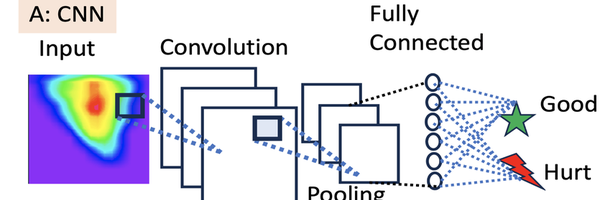
Our goal is to detect hidden hearing loss in a clinical setting. Due to the nature of the sophisticated mechanisms of neuronal response and the complicated multi-dimensional data, we hypothesize that machine learning algorithms, in conjunction of appropriate biological interpretations, can provide insight to detect and calssify hidden hearing loss. Specifically, the methodology involves utilizing a Convolutional Neural Network (CNN), displayed in the above Figure Panel A, to train a classifier distinguishing pre- and post-exposure using input data as images. This allows detection of hidden hearing loss, which has been previously impossible.
However, clinically, it may be infeasible to test the entire auditory receptive field. Thus, we wish to minimize the range and spectrum for clinical tests. To solve this problem, eXplainableAI (particularly GradCAM) is used to identify the spectrums (amplitude and frequency) that are more informative to the classifier when distinguishing between pre- and post exposures. The eXplainable AI (XAI) allows us to decipher the CNN and reveal more information about the detection of hidden hearing loss. In the above Figure, Panel B, the idea behind GradCAM is shown. For the picture on the right, some model may classify it as a cat, the spots highlihged in red are the most informative components supporting this decision. Some other model may classify it as a dog, then the other spots also highlighed in red are the components supporting the alternative decision.
Research
Preliminary Results. Last year, I built up solid foundations which will provide the necessary components to carry out this year’s proposed analysis. The computer code for data processing and statistical analysis (in Java) and visualization (in R) are freely available on my GitHub: https://github.com/ZhouLongCoding/sound_waves.

First, since the raw data is in a binary format (specifically little-endian float), I have developed Java code to convert the data format into plain text to facilitate further processing. Second, since there is unwanted noise and outliers in the data, I have developed Java code for smoothing the data. Third, based on the biological and physiological interpretation from my supervisors, I have developed Java code for feature selection. (In Figure 2, ideas behind each feature are visualized and their detailed descriptions are in the figure caption). Fourth, I have developed R code to visualize the above-extracted features in the format of heatmaps and contour graphs to contrast their values in pre- and post- exposure conditions.

Fifth, rigorous statistical tests were implemented to quantify the significant levels of the scenarios in which the different between pre- and post-exposure conditions are visible. I chose to use paired t-tests [6] to compare the means as well as the Cochran-Armitage Trend Test to examine whether there is an associated trend [7]. Fisher’s Method [8] is used to combine the significance level of multiple experiments. Bonferroni correction [9] on p-values is applied to adjust the multiple test issue. We discovered hearing loss in terms of the dysfunction in neuronal responses to the following aspects: (1) the ability to capture weak signals, (2) overreaction to strong signals, and (3) the ability of distinguishing between noise and signals [2].
Current Project Research.
In my project this year, machine learning algorithms were used to further characterize the interplay of related features. Particularly, Convolutional Neural Network (CNN) is used to train a classifier. The Figure below presents the final form of my CNN in terms of its hyper-parameters through network configurations, training parameters, data processing, and model summary. For all samples, a loss function and a accuracy graph are generated. A sample of such graphs are listed below as well.

Data in Time point 0-9 and 50-99 are known (biologically) to be noisy. I used this prior knowledge to analyze potential overfitting in the training process and select the best model. First, when trains all data jointly, the accuracy in the range of T=10 to T=49 indeed are better (Panel A). Second,when trained individually, the advantage of T=10 to T=49 are more pronounced (Panel B). Third, when analyzing the data jointly for T=10 to T=49 (Panel C) and T=0 to T=9 and T=50 to T=99 (Panel D), the performance of T=10 to T=49 are way better, replicating the patterns observed in Panels A and B. The above observation shows that the model is no overfitting (because of the poor data serve as controls) and we should use only T=10 to T=49 for further discoveries.

Data
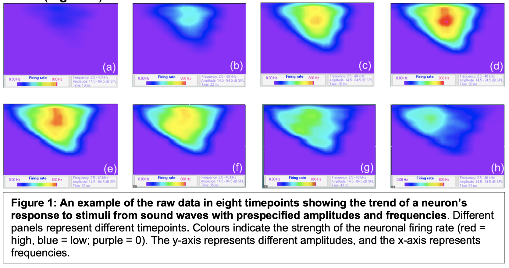
The input data. The raw input data was generated using established methods in Dr. Yan’s Lab [5]. In the wet bench experiment conducted by Ms. Wenyue Xue, a mouse is fixed on the bench, and then exposed to a pre-specified pure-tone sound with 60 dB for an hour (representing the “moderate sound”). Before and after exposure, the auditory neuron’s ability of responding to external stimuli is assessed by specific equipment for 100 ms utilizing various values of amplitude and frequencies. (More specifically, the amplitude is set to be 36 values from 14.0 dB to 86.0 dB; and the frequency is set to be 21 values from 2.5 kHz – 40 kHz.). These experiments were carried out using 20 different mice. The data will look like a series of heatmaps representing the neuronal firing rates under different stimuli (Figure 1).
The output data is dipicted in the figure below. Each small panel in the array is the GradCAM results for an individual sample. The color shows how much "attention" the CNN has spent on the spot, i.e., the importance of the spot that leads to the classification. By averaging all the GradCAM results, I achieved the larger panel showing the ultimate sensible ranges. This outcome paves the path for future clinical test.

Conclusion
The data generated in my project shows the following: First, hidden hearing loss is significant and can be caused by safe sounds, specifically the 60 dB exposure. This is shown rigorously by the statistical tests. Second, I trained a convolutional neural network to detect hidden hearing loss exists in a sample. Finally, I identified the specific range of Amplitude/Frequency that is the most informative in distinguishing pre- and post-exposure, laying the path for clinical tests.
The main innovation of the project is to extract the specific ranges using CNN + GradCAM. The impact is to create a clinical test that may be used for human test. In clinics, two obstacles exist: first, there is no paired pre- and post-exposure conditions to be compared -- we only know the current status of an individual and need to decide by such a single sample. Second, limited clinical resources may allow only a specific ranges to be tested, instead of the full spectrum. My CNN-bsed machine learning classifier solves the first problem and the GradCAM-based eXplainable AI technique solves the latter.
Citations
[1] M. Charles Liberman, “Hidden hearing loss: Primary neural degeneration in the noise-damaged and aging cochlea,” Acoustical Science and Technology, vol. 41, no. 1. 2020. doi: 10.1250/ast.41.59.
[2] Z. Long, “Revealing Hidden Hearing Loss Caused by ‘Safe’ Sounds,” 2023. Accessed: Dec. 14, 2023. [Online]. Available: https://github.com/ZhouLongCoding/sound_waves/blob/main/FinalWrittenReport_size_reduced.pdf
[3] C. M. Bishop, Machine Learning and Pattern Recoginiton. 2006. .
[4] A. Barredo Arrieta et al., “Explainable Artificial Intelligence (XAI): Concepts, taxonomies, opportunities and challenges toward responsible AI,” Information Fusion, vol. 58, 2020, doi: 10.1016/j.inffus.2019.12.012.
[5] R. Bishop, F. Qureshi, and J. Yan, “Age-related changes in neuronal receptive fields of primary auditory cortex in frequency, amplitude, and temporal domains,” Hear Res, vol. 420, 2022, doi: 10.1016/j.heares.2022.108504.
[6] P. G. Hoel, “Introduction to Mathematical Statistics.,” Economica, vol. 22, no. 86, 1955, doi: 10.2307/2626867.
[7] P. Armitage, “Tests for Linear Trends in Proportions and Frequencies,” Biometrics, vol. 11, no. 3, 1955, doi: 10.2307/3001775.
[8] R. A. Fisher, “Statistical Methods, Experimental Design, and Scientific Inference.,” Biometrics, vol. 47, no. 3, 1991, doi: 10.2307/2532685.
[9] S. Lin and H. Zhao, Handbook on Analyzing Human Genetic Data. 2010. doi: 10.1007/978-3-540-69264-5.
[10] A. Chaudhary, K. S. Chouhan, J. Gajrani, and B. Sharma, “Deep learning with PyTorch,” in Machine Learning and Deep Learning in Real-Time Applications, 2020. doi: 10.4018/978-1-7998-3095-5.ch003.
[11] L. McInnes, J. Healy, N. Saul, and L. Großberger, “UMAP: Uniform Manifold Approximation and Projection,” J Open Source Softw, vol. 3, no. 29, 2018, doi: 10.21105/joss.00861.
[12] L. J. P. Van Der Maaten and G. E. Hinton, “Visualizing high-dimensional data using t-sne,” Journal of Machine Learning Research, 2008.
[13] H. Robbins and S. Monro, “A Stochastic Approximation Method,” The Annals of Mathematical Statistics, vol. 22, no. 3, 1951, doi: 10.1214/aoms/1177729586.
[14] S. M. Lundberg and S. I. Lee, “A unified approach to interpreting model predictions,” in Advances in Neural Information Processing Systems, 2017.
[15] S. M. Lundberg, G. G. Erion, and S.-I. Lee, “Consistent Individualized Feature Attribution for Tree Ensembles,” ArXiv, Feb. 2018, Accessed: Dec. 14, 2023. [Online]. Available: https://arxiv.org/abs/1802.03888 [16] S. Ben Jabeur, S. Mefteh-Wali, and J. L. Viviani, “Forecasting gold price with the XGBoost algorithm and SHAP interaction values,” Ann Oper Res, 2021, doi: 10.1007/s10479-021-04187-w.
Acknowledgement
This work was done during my internship in Dr. Jun Yan’s research laboratory at the University of Calgary. I am very grateful to Dr. Yan for his support throughout the research process. Second, I would like to acknowledge Ms. Wenyue Xue, a PhD student in Dr. Yan's Lab. Ms. Xue generated and collected the experimental data on which I ran my machine learning and statistical methods. Dr. Yan’s research has been supported by the Campbell McLaurin Chair for Hearing Deficiencies and the Natural Sciences and Engineering Research Council of Canada (NSERC).