If a CNN is programmed on Python and introduced to 2000 distinctive images daily, then they are capable of properly identifying malignant tumors within the lungs from Computed Tomography scans (CTs) at a minimum accuracy of 80% in the span of one week because the model would have been trained on a suffiecient amount of data to recognize crucial and relevant patterns in CT scans.

Abstract

This scientific article explores the identification of malignant, cancerous tumors via the employment of Convolutional Neural Networks (CNNs), a deep learning model engineered in Python code. The approach I present develops a machine learning algorithm equipped to attain a threshold accuracy of 80% percent within only one week of training, where each day, the CNN is fed masses of CT scans through the means of user input displayed on a personally constructed website. On a daily basis, measures will be implemented to ensure the refinement of the network in order to guarantee optimal performance and results by leveraging the pattern recognition techniques of regularization, performance indicators, optimizers and data enhancement, each of which will be meticulously documented in the subsequent chapters. The objective of my novel design is to explore and audit the powerful capabilities of CNNs in assisting to bridge the alarming gap in the availability of rapid and proper resources for individuals affected by cancer. This continues to accelerate the process of diagnosis as well as offering medical professionals an additional innovative analysis tool amidst the growing pool of diagnostic frameworks.

1. Introduction

Significant progress has been made with detecting various forms of cancer through the advent of advanced and nuanced technology, namely artificial intelligence (AI). The surge of this tool has led to the augmentation of available programs and algorithms designed to identify a myriad of cancerous cells and tumors, thus offering a glimpse of hope to the lives of those who courageously endure such diseases. Medical practitioners have implemented Computer-Aided Detection (CAD) in the last few years to anatomize medical images, such as CT scans and Low Dose Computed Tomography (LDCT) scans, to find suspicious areas of the body that may indicate the presence of lung cancer. This medical model is a byproduct of recently introduced Deep Learning Algorithms, which require training of neural networks with enormous amounts of data to distinguish essential patterns within said data, or ‘inputs’, in order to form precise predictions and correlations to reach a desired output. Deep Learning Algorithms can be further subdivided into various categories, such as Recurrent Neural Networks, Long Short-Term Memory Networks, and Convolutional Neural Networks (CNN).

For the specific task of detecting cancer within the lungs, CNNs would be considered the preferred form of image classification among these networks, as its primary function is to process data displayed through a particular medium, namely images. It manipulates the information, once it has been transcribed into a computer program, into a myriad of products. These can include but are not limited to classification, segmentation, probabilistic control, and object recognition. The debut of the application of CNN models was just a decade ago, in the early 2010s, demonstrating the possible underutilization of these models to date, as their existence is very salient towards the global effort of cancer diagnosis. In the case of lung cancer detection, CNNs have proven themselves to be so proficient at this task that they have been able to outperform radiologists and several other medical professionals. In 2012, GoogleNet had an astounding accuracy of AI detection with a steady performance of 89%, while the limit of the human pathologists was at 70% (National Library of Medicine, 2012). The essence of this project is to formulate a CNN in a short amount of time, with the primary objective of determining the locality of cancerous lesions found within the lungs, as well as the overall presence of lung cancer, in order to narrow the divide between the attainability of resources capable of conserving countless lives, as well as seeing the true scale of competency that a CNN can possess in such a short period of time.

1.2 Brief CNN Overview and History

CNNs are akin to a work of science fiction, their formidable propensities a testament to the remarkable research and experimentation of data scientists and machine learning researchers over the decades. Their journey commenced in the late 20th century, with the advent of Neocognitron, proclaimed to be the earliest precursor of the CNN by esteemed researchers (Brajesh Kumar, ApplyHigh Blog, 2021). The Neocognitron shared architectural aspects that imminent archetypes would inherit, entailing the application of convolution, pooling layers and feature extraction. This predecessor was inspired by the visual nervous framework adopted by vertebrates [22]. The layers of the Neocognitron employed the alternation of simple cells (S-cells) and complex cells (C-cells) as a primary means of the extraction of features of an input image [22]. A cyclical process would persistently reiterate, where the S-cells would be in charge of selecting local features from their provided output, while the C-cells were engineered with the purpose of accommodating to changes in orientation and position of the data, assumingly to enhance the holistic analysis of the findings. The model built up gradually, as regional traits captured in preliminary stages progressively combined into larger, more global features. Nevertheless, it was limited to the distinction of Japanese characters and various other differentiation assignments.

Following the Neocognitron was the LeNet-5, chiefly refined in between the years of 1989 and 1998, and formulated with the intention of executing handwritten digit recognition challenges. The LeNet-5 was among the first to embrace the widely recognized CNN structure: the model features an input layer followed by convolutional and pooling layers, culminating in a fully connected layer that seamlessly transitions to the output. It employed 5x5 convolution layers, while pooling layers were 2x2 [22]. In total, the LeNet-5 utilized over 60,000 distinct individual hyperparameters to achieve high performances. Hyperparameters of models that call for considerable catalogues of storage, like those of CNNs, prove to be quite cumbersome, but this is an essential consideration when developing any neural network system.

As CNNs continued to advance over the decades, a heighted curiosity regarding their progression and utility materialized. ImageNet large scale visual recognition challenge (ILSVRC) was established in 2010, where researchers in machine learning and computer science continued to pioneer the development of CNNs. In its inaugural year, the leading model achieved an error rate of 28%, representing a significantly lower margin of error compared to prior models. The following year saw researchers improved the score to 25.8%, marking a significant enhancement of 2.4% [22]. In 2012, the collaboration of Alex Krizhevsky and Geoffrey Hinton resulted in the creation of AlexNet, which became the most well-known CNN architecture of its time and remains impactful to the field today. This model achieved a notable error rate of 16.4%, marking a substantial enhancement [22].

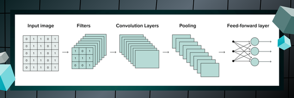
Research of CNNs has revealed the manner in which these networks dissect 2D images and learn relevant features the model deems as being appropriate to the classification of the image. Naturally, computers are unable to ‘see’ the exact way as the human eyes, by virtue of their lack of biological vision as well as contextual comprehension. The familiar ‘binary construct’ is the special ingredient in the recipe of electronic eyesight. Images can be broken down into simple matrices of numbers, as each individual pixel carries a numerical value of a varying degree [18]. The pixel representation as vectors of the input image is then fed into the system followed by additional measures in future layers, that will soon be discussed, in order to ultimately accomplish the intended result. The exact functions of these layers will be detailed in the concepts section of this article.

The future of CNNs is bright, but one crucial issue that should be addressed is the high computational necessities required for the model to function appropriately. Large data assets are a must-have, as the models are prone to overfitting data and acting extremely meticulously, lacking the ability to suitably generalize information. Their sensitivity to discrepancies within findings adds exponentially to their intensive computational consumption, giving rise to the reason for why these systems necessitate such exhaustive and voluminous amounts of data repositories. The objective is to operate smoothly on unseen data, and this target is held for all artificial frameworks, but CNNs have unique conditions that are obligated to be met. CNNs have a high risk-reward construct where the attaining of these circumstances ensures a smoothly running system, rendering them highly effective in image processing, distinguishing this particular algorithm from its counterparts. 

While experimental in nature, this project actively seeks to contribute to the continuously expanding line of work performed on AI models within the healthcare system in order to bring these approaches deemed ‘out of reach’ by the masses to the assistance of the critically ill, as well as to the consciousness of the populace. 

1.3 Background

Nearly 1.8 million people worldwide lose their lives to lung cancer annually [5]. This is a substantial amount of the population that have succumbed to such a dangerous and destructive disease. In Canada alone, an estimated 20 600 people will perish from lung cancer this year, and that number will continue to increase if no steps are taken to alleviate the burden of this disease [2]. Lung cancer is the deadliest and most perilous of all cancers, as it sprouts from one of the most integral organs that the body requires to survive and maintain homeostasis - the lungs [2]. The lungs play a crucial role in the process known as respiration - the transferring of oxygen and carbon dioxide throughout and outside the human body. Our lungs are essentially a filter that removes the carbon dioxide within, a waste that is produced by our blood cells. The carbon dioxide that is diffused by our cells enters the bloodstream and once it has reached the lungs, it is expelled out of the body as a whole from exhalation [6]. As molecules of oxygen infiltrate our system, the alveoli, miniscule air sacs of the lungs, are the first point of contact of the bonds of oxygen, followed by the blood flowing within capillaries lying on the textured lining of the alveoli. After successfully entering the bloodstream, in a matter of seconds, the hemoglobin proteins housed within red blood cells bind with these molecules, 4 oxygen per a single hemoglobin molecule, developing a new compound that voyages through the human body [1], [6].

When the above-described process is interrupted by tumors as a result of cancer, it poses an urgent issue that must be treated immediately. As lung cancer progresses, the tumors affiliated with this type of cancer can block and narrow the airways, making it strenuous for air to flow in and out of the lungs, thus affecting the normal functionality of the lungs. This obstruction traditionally presents symptoms such as wheezing, persistent coughing, and shortness of breath, resulting in serious discomfort to the human body as well as gradual destruction and cessation of adjacent structures. Due to the reduced airflow, decreased oxygen levels in the bloodstream will occur, which in turn can lead to extreme fatigue and weakness. In later stages of lung cancer, the tumors begin to invade surrounding structures, such as the bronchi, blood vessels or the pleura (lining around lungs). This can further cause additional symptoms, namely chest pain and difficulty breathing. However, it is important to understand that there is a varying degree of the impact on respiration according to the location, stage and size of the lung cancer [6]. 

On CT scans, the regression of the lungs are more evidently apparent, as abnormal growths take up the form of irregular or round white or gray masses, while lung nodules appear as minute bold dots on skin tissue of the lung [8]. Despite the fact that there are key components of the imaging that are easy to visualize and distinguish on the part of the radiologists, human errors and flaws are bound to interfere with the ability to properly arrive at an optimal solution and yearned result to effectively corroborate the case of the patient.

The highlighting of the physiology of the lungs has been of paramount priority up to this point. The impact that lung cancer has on human lives, and its effect on human bodies cannot be over emphasized. A point was established earlier that referred to how this specific type of cancer must be handled immediately, and action must be taken very quickly to eradicate the cancer inside of the body. However, how would we be able to ensure early detection of lung cancer and take steps to properly assist patients on their journey back to normalcy within their bodies? This question is routinely pondered upon among medical experts and the general population alike, given the relative 5 year survival rate in Canada is said to be 4%, due to the unfortunate fact that at a minimum, half of the people who contract lung cancer only realize they suffer from the illness by the time that they have been diagnosed at stage IV [2]. For those who are diagnosed at stage 1, which is around 1 in 5 people, their 5-year survival rate is at a higher and superior 63%. To put that into perspective, nearly 50% of Canadians who contract lung cancer and are diagnosed at stage 1, the beginning phases of cancer, pass away within those 5 years, and the survival rate diminishes for each year that passes by [2]. This is where the previously mentioned advances in healthcare that have led to the evolution of current mechanizations becomes relevant, particularly the CNNs that have demonstrated significant promise in refining the precision and pace of early-stage cancer detection.

In the previous section, Computed Tomography (CT) scans, a distinct version of medical imaging, was briefly touched upon, and examples of abnormal results found within the scan were equally alluded to. CT is a term used to describe the x-ray imaging procedure where a combination of x-ray images is prepared by the CT machine with the intention of fabricating sectional images of compositions within the human anatomy. These graphics contain comprehensive information that exceeds the data of a standard x-ray image, as they are digitally organized to construct a 3D overview of the fixed site [7]. In an orthodox x-ray image, a configuration of dynamic energy electromagnetic radiation, with a sharp wavelength situated between gamma rays and ultraviolet rays, permeates the body to arrive at an x-ray detector of digital manufacture, generating a two - dimensional image of solely dense tissues within. CTs follow a similar model, but where their paths diverge is the planes on which they rest on. CT scans necessitate patients lying on a berth atop a circular frame, as an x-ray tube revolves around the individual inside, considering assorted angles, each 2D image possessing a thickness of tissue ranging from 1-10 millimeters [7]. The completion of the rotation is succeeded by an elaborate illustration of the zone under study, relaying distinguishing features to interpreters for the purpose of offering fitting support towards the patient. 

In the case of this project, CT scans display the full outlook of the lungs condensed into an image with a strictly two-dimensional, flat appearance, serving a pivotal role in the identification of early-stage diseases due to the clarity of the images, and the noticeable lack of noise in the scans. ​

 ​

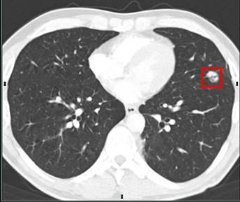
Figure 1.3.1 of CT scan of lungs proven to be positive for cancer

1.3.1. Cancer Growth

Following the heavy emphasis of the grave effects of lung cancer and its low survival rate, this section of the article serves as an insight to the traditional forms of growth that strongly insinuate the presence of cancer of the lungs, founded upon the observations of medical imaging. Even though there is a large multitude of cancers that negatively impact the lungs, medical professionals have classified two main kinds of lung cancer: non-small cell lung cancer (NSCLC) and small cell lung cancer (SCLC) [4]. The more common of the two variants is NSCLC, accounting for approximately 80% of lung cancer cases [4], further subdividing to include adenocarcinoma and squamous cell carcinoma, as well as the additional unique adenosquamous carcinoma and sarcomatoid carcinoma deviants. The opposing SCLC is the more aggressive and difficult category of lung cancer, a cancerous breed that is significantly harder to cure, as they are lung tumors small in size that have already reached various areas of the body. Small cell carcinoma (also called oat cell carcinoma) and combined small cell carcinoma are distinctive varieties of SCLC [4]. SCLC can equally be subcategorized as a limited stage, where the tumor is constricted to one sole lung, similarly situated in lymph nodes near the center of the chest or just slightly above the collarbone. Conversely, extensive stage SCLC has usurped the expanse of a lung, or en route to fully overtake the second lung, the corresponding lymph nodes of the lung, and eventually other vital elements of the body, the latter acts being parallel to the function of a metastatic lung. Metastatic lung cancer begins as cancer initially developing in one lung, however the resulting growth stimulates the widespread of the disease to the neighbouring lung and soon after neighbouring organs [4]. This classification of cancer of the lungs is found to be the most arduous to medicate, as the ever growing field for the demarcation of the illness is only further convoluted when more possible sites are added to the mix.

 

1.4. Perception and Activation Functions

In order to build up to the grand creation of CNNs, it is essential to size down to examine the building blocks of life - the neuron. The brain is a complex system of neurons, transmitters and blood vessels responsible for carrying out the quotidian undertakings at the helm of our very existence as human beings, as living creatures. At the center of the control panel lives the neurons - nerve cells overseeing the transmission of messages between copious instruments of the body that conduct our every move, from breathing to thinking to walking to talking. All that we can and will do is to the grace of an imperceptible cell.

 ​

Figure 1.4.1 Displaying the structure of a neuron

Every single neural network is modeled from this cell structure, replacing the biological nature of the composition with artificial molding. The cell body, or the 'soma' acts as the central part of the neuron, containing the nucleus in addition to the collected signals of the dendrites [23]. The branch-like tendrils of the neuron are the dendrites - extensions with the purpose of acquiring electrical signals of inbound data from vicinal neurons, neurons that are approximately 2 to 5 micrometers distant. The vast majority of input directed towards a neuron occurs on these arboreal structures - by way of the dendritic spine [23]. The final main construct of the nerve cell is the axon - a thin, sinewy fiber of substantial length stemming from the cell body responsible for the transmission of electrical impulses to other neurons for the purpose of circulating new information throughout the confines of the brain and beyond. Most neurons of the human nervous system possess one sole axon obligated to fulfill this function, nonetheless, they offset this confrontation by sustaining ample branching, thereby facilitating communication and interaction of numerous target cells that are contingent upon information that maintains physiological equilibrium [23].

Artificial neurons follow this fundamental program of life, revamping the dendrites into the inputs and weights, followed closely by a summation, which behaves as the soma, and ultimately the output to replace the axon. This is what is known as the 'perceptron' - the building block of neural networks [11]. We take x, our inputs, data sent to the neuron and multiply the value by the corresponding parameter, or weights w. An additional parameter is added into our sum, which is known as the bias b, a specification that adjusts the conclusive rendition of the output so as to equip the algorithm to better match the data and refine predictions, particularly in cases where the input features equal zero. Without this imperative metric, the network will always predict an output of absolute zero when the input is zero, hindering the ability of generalization and inference that a learning model demands in order to thrive.

Once the summation of the weights, inputs and bias has been accounted for in our perception, it is then run through a nonlinear function, a function that mimics the nonlinear order of the real world in theory. The perception is the basest level form of a neural network, and the simplest manner of visualizing deep learning. Perceptions are equivalently hindered by their simplistic origins, whereas their pioneering mechanical counterpart, the sigmoid neuron, overshines the simple structure in most aspects of machine and deep learning [10], [16].

 

 1.4.1. Sigmoid

Sigmoid neurons pick up from where the perception left off, accentuating the presence of the nonlinear function to generate a smooth output between 0 and 1 as a consequence of the sigmoid function. The sigmoid function is a machine learning technique that squishes the output to a value between 0 and 1, advantageously portraying probabilities as binary classification as in alternative to the static booleans of the perception (output is either 0; False, or 1; True). In advanced mathematics, the function is visualized as an S-shaped curve that gracefully traverses the x-axis (representing input) and the y-axis (representing output). The sigmoid function exhibits a monotonically increasing behavior, where the output rises in relation to the input [10].

The function is displayed as this:

 

​Figure 1.4.1.1. Displaying the sigmoid function

   -  The sigmoid function in opposition to the step function (perceptron).  -   ​

​Figure 1.4.1.2. Displaying the sigmoid function on a graph                                        Figure 1.4.1.3. Displaying the step function on a graph

 

1.4.2. ReLU

In the specific case of CNN models, the use of the ReLU function proves itself to be an even more efficient activation function when compared to the likes of the sigmoid and perceptron. The complexity of CNNs requires computational efficiency and data sophistication with the aim of certifying the reliability and ease of the machine. Since the values of the inputs passed through the sigmoid operator are squished between the range of 0 and 1, a significant portion of the initial data will be absent [10]. As the model advances through the values of the inputs, the derivative of the function decreases in volume, marshaling the eventual vanishing gradient problem during processes of model improvement, such as backpropagation [10]. ReLU differs from Sigmoid by means of properly addressing this issue through the model's consideration of the true values of the inputs, utilizing a maximum operation feature that maintains a continuous positive gradient for inputs that return positive values and a reaction of zero for all negative activations from the input [10]. The reasoning behind this approach is to reduce the gravity of unnecessary weights that would have carried negative values so as to remain at a state of uniformity, dissolving the overinflation of weights that would have appeared with more prominence to the CNN. In the eyes of the model, negative values share the exact worth as values of 0, as there is a lack of activations with respect to the weights to carry unto further layers, so the elimination of negative values equally terminates unwanted exceptions that would have brought an auxiliary sense of difficulty to the managerial apparatus of the program.

This method is glaringly less computationally heavy and reintroduces the understandability and simplicity of the perceptron once more. Simplicity is an extremely valuable sought-after asset in order to increase productivity and efficiency, especially taking into consideration the limited period of time available to engineer the model in our experiment.

 

1.5. Computing Loss

In order for a neural network to aptly learn, it is essential to teach the model the cost to be incurred from incorrect predictions. If the algorithm was left to self-predict, it would deliver nonsensical outputs for as long as each iteration continues, as there is no means of conveying the fact that the predictions of the network are erroneous. To quantify this loss, we can follow a plethora of formulaic expressions to measure the difference between the forecasted output and the actual output value. The general term for the measuring of the total loss accounted for in the entire dataset would be classified as Empirical Loss. Empirical Loss pertains to the efficacy of the model with respect to the predictions that it created and how accurate those projections came to be when juxtaposed with the true values. The alternate expression that still uses the initial ‘Empirical’ title is Empirical Risk [10],[18]. Even though their distinctions appear to be inconsequential, empirical risk describes the identical central notions, but stress is applied on the theoretical circumstances to explore possible losses over the arrangement of data [24]. To observe our loss, we can follow this blanket formula that serves as the foundation for all lost functions. This function grants us the ability to examine the true performance of the network while it undergoes the training stage:

​

Figure 1.5.1  Displaying the cost function neural networks manipulate for the quantification of loss

A very common loss function popular among developers of CNN models is Binary Cross Entropy Loss (CEL). This particular loss function evaluates the capability of a model concerned with classification through probabilistic terms. The measure outputs a probability output between 0 and 1, where 1 is of positive nature while 0 leans towards the negative activations. In code, the softmax function directly apprises the programmer of the validity of the network through detailing the distance of two probability distributions, as well as comparably reporting on how deficient the model to facilitate the proffering of critique the model receives [17], [18].

​​

 

​

Figure 1.5.2. Illustrating the equation of Binary CEL responsible for system penalization

 

The penalization of faulty predictions is integral in the computation of loss in our model so as to escort the model in the journey of synthesizing outputs that reliably connect a particular instance to a certain category. In due course, the loss of the algorithm remains committed to declining in value, as the model adopts new tactics through learning to arrive at a target state. This approach is labelled as loss optimization.

 

1.6. Loss Optimization

From the criticism that has been received from the loss function, we can procure an appropriate course of action to optimize the network through the channel of weight optimization that achieves the lowest possible loss in our network. We should aim for an enhancing channel that represents the most favorable weights as being equivalent to the weight values that greatly curtail the cost function, such as the following:  

 

​

Figure 1.6.1. Equation of loss augmentation function with defined values

 

Gradient Descent, a mathematical algorithm that maneuvers the cortex function in order to satisfy the demands of the network with respect to its individual weights, is heavily applied on CNN models in addition to other deep learning architectures. There are varying designs of Gradient Descent algorithms, such as Stochastic Gradient Descent that will be unraveled in the following paragraphs of this article, and the sophisticated adaptations that emerge from this function. We can physically visualize this process using a three-dimensional coordinate system, where we select an initial, or a point on the plane, entirely arbitrarily, so as to give the network the opportunity to efficiently learn without any original partiality or predisposition [10]. The method of initialization varies on the specific network, but since this article primarily focuses in CNNs, their system operates on a ReLU nonlinearity function, requiring the use of He initialization, a mechanism for establishing weights that deliberately scales the variance of these weights, resolving the issue of a possible fixation at zero where the network fixed at zero output. 

He Normal initialization entails the extraction of initial weights from a normal distribution, usually a Gaussian distribution, with the discrepancy sized by 2 to account for ReLU neurons that have fifty percent of neurons output values of zero [25]:

​​​

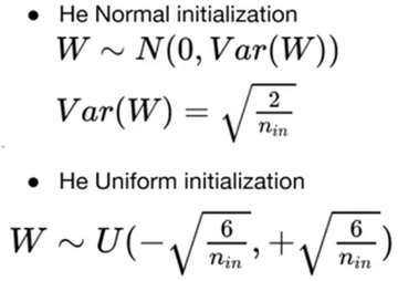
Figure 1.6.2. He Normal and He Uniform Initialization in Machine Learning

 Following our activation of our weights during gradient descent, we compute the gradient at that position utilizing the partial derivatives of our loss function J(W) and our weights W for a local estimate of the slope expansion as well as decrease with the following expression:

Figure 1.6.3. Depicting the weights on a slope expansion

The subsequent step at our gradient computation is to proceed in the opposite direction of our gradient, as it is informing us on the trajectory of loss growth, and our objective is to fully minimize our loss to attain a value of zero for our loss function. The opposite direction of our gradient is down, so we step down into the landscape, adjusting our weights accordingly [18].

This process is to be repeated until a point of convergence, a point that is known as a local minimum, where the loss function is at its lowest value in the particular area of our landscape.

​

​

​1.6.1. Stochastic Gradient Descent:

Traditional Gradient Descent accounts for the entire dataset during the process of weight refurbishment, implying that the adjustment of weights will take place only once the model has reviewed all available data. This inopportune and burdensome scheme can prove to be quite prolonged and numerically demanding, necessitating a continuous influx of data before any weight adjustments can enhance the system's performance. If our objective is to develop a program within a week, this configuration is far from optimal. Extended training durations may overwhelm the system, such as a computer, that hosts the program. Stochastic Gradient Descent (SGD) introduces a new concept known as batches, where single data points are implemented one at a time to compute our gradient as well as update the weights of the network. This combats this substantial concern by offering quicker convergence rates and stochasticity that can prove to be quite beneficial for a learning model [10]. SGD obeys the same phases of regular Gradient Descent, but with some crucial differentiations:  

1. We initialize the weights haphazardly while considering the He initialization function
2. We loop this discrete process, with new additions, until convergence:
   1. Select a sole data point of variable i - a batch of certain points
   2. Then compute the gradient - ∂Ji(W) / ∂W
   3. Adjust and update the weights accordingly -  W <- W - η * ∂J(W)/ ∂W
3. Thereafter, we return our weights to be optimized later on.

Unfortunately, an expedited approach has associated disadvantages. SGD does bring noise, or haphazard gradient estimations into the optimization of weights as the method of updating weights one batch at a time does not leave much room for precision and total order [10]. This algorithm counters this downside with the prominence of the learning rate, an adjustable parameter that corresponds to and regulates the value of the weights during training. This system of improvement will be elaborated upon in further discourse within this article.

 

1.7. Backpropagation

The upgrading of our weights first begins once we understand the gravity that each weight holds pertaining to the gradient of our loss. When we go forward in a neural network, we commence with our input of variable x, followed by the strength of the connection which is defined by our weights, of variable w, towards their combined summation by an activation function in a hidden layer [10], [11], [18]. The power of the connection between this layer and our output is equally determined by the weights of this layer. This process allows us to feed the data of the initial input neurons to the remaining neurons of the output layer. Backpropagation reverses this pattern, with the aim of computing the gradient, or the slope of the loss function in relation to the weights of the system, modifying the corresponding strengths between the layers in the model. In order to realize this goal, we can apply a chain rule commonly found in calculus to soon individually update the weights, using the partial derivatives of our output and weight parameters:

​

Figure 1.7.1 Depicting the chain rule, the essence of backpropagation for neural networks

 

The use of partial derivatives assists in our understanding of the correlation between the changes in the cost function and each parameter W, as this function has hundreds of parameters that impact the approach the model acts on. Partial derivatives account for only one variable in the derivative while preserving the others as constants: unchanging values [10]. In each iteration of the chain rule, the weights are updated in the exact direction of the negative gradient of the cost function to minimize the total loss of the model, as well as to learn from previous errors in the output layer [18]:

​

Figure 1.7.2 Depicting the chain rule with the addition of weights from summation layers (z)​​

 

Backpropagation is crucial in understanding the role that each individual weight plays in the errors of the output, advising us on what specifically requires change in our network and the scale of which that change is mandatory, but it does not indicate the size of the update for each weight. That is where the learning rate comes in to fully complete our weight optimization while considering the advice of the backpropagation process.

 

1.8. Learning Rate

Our learning rate determines the magnitude as well as proportions of the meliorations the model received from backpropagation. The setting of the learning rate is an extremely difficult task to accomplish due to the complexity of neural networks, and subtleties that each network carries, bringing rise to slow conversion in small learning rates and overshooting in large learning rates [11]. In order for us to select a proper learning rate that accommodates to our model, we have two main choices:

1. Experiment on several different learning rates to see which one works the best, or,
2. Engineer a flexible learning rate that revamps according to the landscape of the model.

 

This option alleviates the burden of finding an exact learning rate that meets the exact needs and requirements of the system and instead replaces them with an intuitive mindset to match the environment of the network, depending on various factors unique to the model. These facets may include the proportions of the gradient, the speed of learning and the magnitude of the specific weights. Luckily, the programmer is not required to manually address these considerations, as we can import adaptive learning rates responsible for the automatic adjustment of the learning rate derived from the strength each parameter carries on the gradient. Some of these algorithms include:

 

• Adam                                                  tf.keras.optimizers.Adam
• Adadelta                                             tf.keras.optimizers.Adadelta
• RMSProp and,                                    tf.keras.optimizers.RMSProp
• Adagrad,                                             tf.keras.optimizers.Adagrad

 

where each follows a similar TensorFlow implementation in Python.

With our learning rate set to account for all the refinements of our model, we can guide our network smoothly through the training process to develop functionally and thoroughly.

 

2.1. Models in Practice

Our model has now reached a point where it can be exposed to new data, and we want it to recognize patterns in data it has not previously been exposed to. There are three possible ways our model may act based on how it reacts to features: 

1. Underfitting: The neural network has not reached the point where it can fully comprehend the data and make connections of the features to what was trained on.
2. Overfitting: The neural network has learnt all the supplementary complex parameters that prohibit the model from generalizing, instead it concentrates on detecting extreme patterns that are too niche
3. Quintessential: The model can identify patterns in the data to match the features of the information it received from the training phase.

So, how can we ensure that our model always meets the ideal fit to avoid underfitting and overfitting the data?

 

2.1.1. Regularization

The process of learning is done through the means of training and testing, this being the rudimentary format for all forms of learning for all intelligence. During training, we can leverage a technique that impedes our model from overfitting through the means of penalization, mirroring the practices of the softmax function highlighted earlier. This technique is classified as Regularization. Regularization builds unto the loss function by adding slight modifications, through the inclusion of a regularization term. 

Figure 2.1.1.1. Depicting comparing the loss function with L1 regularization to without L1 regularization

The value of these terms vary depending on the targeted method, however, there are two main deviants that parallel the risk functions of Mean Absolute Error (MAE) and Mean Squared Error (MSE), where for a MAE is a measuring function that determines the mean, or average volume of the absolute value of errors between the predicted and actual output, and where MSE acts as an estimator deviation that exploits the averaged squared summation of the errors between the predicted and factual values. They consist of L1 Regularization, and L2 Regularization. 

L1 Regularization accounts for all the values of the weights to the absolute value, joining them together with the loss function. This strategy is prone to inadequacy, as some weight values settle at exactly zero, lacking overall depth and essential distinction. Fortunately, L2 Regularization mitigates this dilemma through squaring the values of the weights, shifting them closer to zero but never towards the exact value of zero. This approach enables larger weights to be more prominent compared to the vast sea of nearly null but still relevant values, guaranteeing that every weight retains its importance. With our regularization term now specified, the next proceeding required on the endeavor towards overfitting prevention is to pinpoint a system stemming from Regularization that demonstrates the highest level of excellence in obstructing the model from overcomplicating the details in the data alongside refining the generalization of the model [9],[14].

 

2.1.1.1. Dropout

The objective of the Dropout methodology is to erratically set a handle of pertinent activations in the model to zero during training, with the intention of intuitively guiding the network to establish a myriad relevant connections in its complex on its own accord, without the aid of outside support. The lack of certain activations forces our network into a position where it needs to widen its scope of reliance on a particular node or a small quantity of nodes in the hope of weakening established links in the network that relentlessly provoke overfitting.

2.1.1.2. Early Stopping

This subsidiary approach of Regularization involves the termination of the training of our model exactly before the model has the chance to overfit. By and large, the model commences the training process while undercutting, with our loss function at its highest point in training. As the model becomes more accustomed to the feed data, it picks up on correlations that it would initially skim over. All of this is occurring whilst our loss persists on its declining pathway through gradient descent. As soon as we perceive a change in the hyperparameters of the model that acts as a strong indication towards a trajectory of overfitting, we terminate our training process, and assess the capabilities of our model on new, unseen data in order to appropriately maximize the generalizability of our model.

 

2.2. Image Preprocessing

Earlier in the research section of this article, I gave a brief overview of computer vision and how it specifically pertains to the fundamental makeup and essence of CNNs. CNNs essentially consist of matrices of individual numerical vectors, each with proportions dictated by the model. Images in their most natural form are composed of the same structure - geometric values held in the confines of pixels. Monochrome images can be represented by matrices in the second dimension, referring to the proportions of height and weight, and they are equally displayed in pixels of differing luminosity, from a scale of 0 to 1. Colored images add an additional aspect of dimensionality, where they upgrade to a three-dimensional matrix to represent height by weight by three for each individual pixel. The value of three represents red, green and blue, the traditional color scheme that our eyes process information through [14]. These values are transferred through the network to accomplish the goal of either classification or regression. CNNs have the purpose of assigning the probability of the features of belonging to a particular class. The determination of the class is based on key aspects of the input that implicate a specific connection to a certain class. These aspects are correctly termed as features. Features allow models to identify characteristics of the data that relate to a sought-after image category. Once the features of a particular class are picked up by the network, it would naturally deduce the given data is of that class. To illustrate, key features that the programmer might explicitly mention for lung cancer detection by the model could include regions of the lungs that are most sensitive to cancer on the scan, as well as the presence of abnormal white spots. These details empower the model to infer accurate class forecasts. This example would also be a demonstration of manual feature extraction, where the model is being informed on certain features to be vigilant about. Nevertheless, manual feature extraction arouses major challenges, as features that the model should have registered were dismissed due to certain criteria that might encompass, scale variation, background distraction, deformation, occlusion, and most significantly, intra-class variation. To mitigate this issue, we can construct a feature hierarchy extracted from the data to arrive at our anticipated result. This feat can be accomplished by dividing the complexity of features into three levels: low-level features, mid-level features and high-level features.

 

2.2.1. Low Level Features

In the case of lung cancer identification, our primitive features would incorporate texture, the visuals of lung structure, surrounding areas, and any irregularities in the imaging data, edges, the boundaries of certain elements, and corners, the representations of basic shapes that may help to discern tumors and components of the lungs apart. These features present as the first qualities dissected in the beginning layers of the CNN to raise any concerns regarding the presence of cancer. CNNs and other analogous paradigms really heavily on the concept of attention, the relevant important of a distinct element, to decide an adequate course of action to execute the given endeavor. Low level features hold the most magnitude, as they act as the determinant for the direction of our model, and even though it does not entirely establish the full panoptic depiction of our input, these factors exert influence on the focus of ensuing layers.

 

2.2.2. Mid-Level Features

Our mid-level features begin with the combination of the features that originated from the previous layer to uncover intricate patterns that could be associated with formations and anomalies that prove to be complex. This involves, but is not limited to, variations in density levels that might stipulate the existence of tumorous tissue, and nodule shapes that exhibit cancerous characteristics. This idyllic result exclusively transpires once the model has familiarized itself with the innate sophistications of the previous data given to associate such complicated links instead of the customary nonsensical output.

 

2.2.3. High-Level Features

Our concluding set of features unite the observations that preceding layers uncovered, assembling elaborate designs to develop a comprehension picture of the data provided. Tumor boundary delineation, where the model can distinguish tumor boundaries from surrounding tissue, along with nodule categorization, where the network recognizes the difference between malignant and benign nodules, so as to maintain clarity between the two masses, are the two leading elements of advanced feature extraction in our network. They act as the final assessment of our input image, determining the ultimate batch of features the model takes into consideration for the classification. Each of these sets of features are captured within a vector of pixel values, where in some models, all neurons possessing the values of these vectors are connected to a single neuron in the hidden layer. In theory, this scheme seems ideal, as the value of all the previous neurons are held in one single neuron of the hidden layer instead of the neurons being aligned with countless dissimilar inputs. Nonetheless, the network no longer retains the intricate structure of the initial images, forfeiting all spatial information while adopting the weight of immeasurable parameters that each neuron held. In lieu of overlooking the importance of spatial structure in our input, how might we utilize this framework to rebuild the composition of the image in a manner that our model can comprehend? This is where the concept of aligning patches of the input to the neurons of the hidden layer. 

 

2.3. Convolution

This extraction of features is known as convolution, where our sliding window, or filter, is composed of a set of weights, each responsible for regional feature dissection of their designated input section to be shifted by 1 pixel for a subsequent patch [18]. Once we have slid a filter to a certain section of our image, we perform element-wise multiplication, where we multiply each corresponding match of elements, and affix our outputs, seamlessly producing a feature map [18]. 

Figure 2.3.1. Displaying the perpetual cycle of convolution and filtering

These filters are implemented to encourage algorithmic efficiency and ease in opposition to the procession of individual pixels. Our convolution operation can be recorded as the following (for the instance of a 4x4 filter):​​

Figure 2.3.2. Converting the convolution operation as a mathematical expression

​​where the summations amount over the indices i and j from the range of 1 to 4, Xi + p,j +q act as the input of previous layers, b acts as our bias, and Wij are the weights [18]. We can describe this expression as the weighted sum of the weights of the filter and the corresponding input values.

Convolution allows room for the preservation of spatial information due to the fact that it does not thrust all the values into one large matrix storing all the values of the features from the input. Neurons in the hidden layer is the weighted sum of the inputs with an additional bias term, acting as a counterbalance to guide the model in their decision-making even when the activations of the input are zero. Following this, we apply an activation function upon each neuron to offer solely non-negative values. The motive of this application is to reduce the gravity of unnecessary weights that would be carried negative values so as to remain at an equilibrium, so as to not excite the overinflation of certain weights that now appear to be more important than their true nature, as we have previously mentioned.

 

2.4. CNN layers

A single convolutional layer can be presented as a three-dimensional object, with dimensions of height, width and depth (h x w x d) [14]. The height and width of a CNN layer represent the spatial dimensions of our features we were formerly seeking so hard to conserve, whereas depth embodies the number of filters in a given layer [14]. The designation of the step size of a provided filter, or the speed of the filter slide, is denoted as a stride by all CNN algorithms. The specific region the neuron in our hidden layer is processing from the input feature is routinely titled the receptive field, determining the context a neuron receives when choosing features to address in following layers. In a CNN, the receptive field starts small in the first layer and gradually grows larger as the network deepens, with each layer building on the outputs of the previous one. This allows neurons in deeper layers to capture information from progressively larger portions of the input image, causing the receptive field to expand.

 

2.5. Maxpooling

In order to reduce the immense dimensionality of our feature maps, we can leverage a process known as Maxpooling to extract the highest, or maximum value of every patch engineered by the filters to the succeeding layer [14]. Maxpooling facilitates the minimization of the amplitude of the features, permitting the lack of an overabundance of hyperparameters, as well as the maintenance of spatial constancy [18]. Pooling is the final step in the cycle of feature learning, and our process of the interchange of convolution and pooling repeats until a point of satisfaction, where we have reached the tip of our hierarchy of features to output the final advanced level features. This new undertaking is the second major component of a CNN model - classification.​​

Figure 2.5.1. Visually presenting the process of maxpooling in CNNs ​​​

2.6. Classification

Once the advanced level features of the previous layers concentrated on feature extorsion have been outputted, the product is flattened into a one-dimensional vector, cleansing the output of previous spatial depth be interpreted by the final fully-connected layer, or the ‘Dense’ layer as recognized by Python code, which utilizes said features for our image classification [14]. This is where the model calculates the particular class the input image is linked most strongly with. The classification of our input image is expressed in the form of a probability, where the model responds to the main query of ‘how likely this image depicts the presence of cancer’ [18]. In order to properly convert the output into a likelihood, we can operate the sigmoid function, transforming the set of values into probabilities between 0 and 1, equally establishing the presence of a binary classification system once we have the objective of only possessing two possible outputs. If there were multiple classes that existed for the model to select from, the softmax function would be the operator of choice, transfiguring the output into probabilities corresponding for each class, corroborating the notion that the total sum of probabilities across all classes equals 1. On Python code, we can compile everything and outline our convolutional neural network by describing the layers as follows [20]:

 

# Create and compile the CNN model
 

def create_cnn_model(input_shape=(IMAGE_HEIGHT, IMAGE_WIDTH, 3)):
    model = tf.keras.Sequential([
        tf.keras.layers.Conv2D(32, (3, 3), activation='relu', input_shape=input_shape),
        tf.keras.layers.MaxPooling2D(pool_size=(2, 2)),
        tf.keras.layers.Conv2D(64, (3, 3), activation='relu'),
        tf.keras.layers.MaxPooling2D(pool_size=(2, 2)),
        tf.keras.layers.Conv2D(128, (3, 3), activation='relu'),
        tf.keras.layers.MaxPooling2D(pool_size=(2, 2)),
        tf.keras.layers.Flatten(),
        tf.keras.layers.Dense(128, activation='relu'),
        tf.keras.layers.Dense(1, activation='sigmoid')
    ])
    return model

…

 

# Last dense layers for classification

dense_output = Dense(128, activation='relu')(cnn_output)

final_output = Dense(1, activation='sigmoid')(dense_output)

 

This block of code is the compulsory archetype for the CNN model structure specifically, excluding the other aspects of the code that enable the CNN model to unleash its full potential. This prototype empowers these neural networks to thrive in scores of professions and fields, such as medical cancer screening, for cancer classification, object detection in terms of cancer localisation, and segmentation, where in a diagnostic vantage point, the constituents of a particular region of the body are individually identified and recognized, say through the means of recurrent non-invasive visualization methods. 

 

 

 

3. Variables

These variables are specific facets of the experiment that will contribute to the overall outcome and whether or not the hypothesis I crafted is in strong accordance with reality or with fantasy.

3.1. Responding variable

Accuracy:

• The responding variable that acts as the ‘effect’ would be the outcome and precision of the CNN, such as whether or not it can accurately predict the presence of malignant and benign tumors in the scans. The accuracy of the model will be measured by diving the number of correct predictions by the total number of predictions made for each day in order to determine the accuracy of the model for each day of the experiment. 

3.2. Manipulated variable

Computed Tomography (CT) Scans:

• The manipulated variable is the two categories of the images fed into the CNN: cancerous CTs and non-cancerous CTs, formulated to give the end result that checks the validity of my hypothesis. I created a folder housing the two CT scan variants, which are further subdivided into Adenocarcinoma, Large Cell Carcinoma and Squamous Cell Carcinoma under my 'Malignant Tumour' bracket. This is in order to see how the model reacts to various manifestations of data during training, validation and regular testing.

Hyperparameters:

• Vital contributors to the outcome of the model, such as learning rate, batch size, epochs, number of layers, model architecture, regularization and data augmentation will all be tuned in various ways to give the model the necessary resources to flourish and adapt at a rate that ensures the best possible outcome.
• Weights never stay constant, as the value and strength of each connection between neurons is consistently updated depending on the judgement of the network. These adjustments will be documented in order to observe their individual effect on the products of the experiment.

3.3. Controlled variable

# of Images:

• The quantity of images fed each day (~20 000 - but there are 2000 different images that are reused to add up to the value of the range of 20 000) will continue to remain static so as to remain at a constant rate of image exposure, preventing any irregularities in the performance of the CNN due to fluctuating training data. 

Programs used:

• I will be utilizing the softwares of Vscode, Windows Notepad, and GitHub for my coding which will be employing the overall program of Python.
• The additional administrator programs used will be Windows PowerShell, and it will be the only computer administration program used to limit my code activation to one environment. PowerShell leverages the functions of Command Prompt, another administrator available on my computer, with additional, more complex features.
• However, the software I will be using for my online app will be Streamlit, but the code for the app will continue to be implemented from Python.

Time Frame:

• Maintaining the one-week time frame is a fundamental component of the experiment, given that the basis of the project is to assess the potencies of CNNs in a defined length of time. Adding more or less time would greatly impact the overall outcome of the venture.

4. Procedure

Below is a detailed course of action descriptively detailing the specific exploits that led me to my desired outcome.

4.1. Code

• To commence, select an IDE program, such as Vscode or Notepad, to use as the development of the software of the CNN.
• Create an umbrella folder, one that will be responsible for housing all the information, scripts, Python environment and extensions of the experiment.
• Within the folder, add three more secondary folders for code environment (myenv), and a folder encompassing all the scripts and data for the app, which can be appropriately named streamlit_project, as a nod to the application overseeing the presence of the model.
• Once most of the settings have been attended to, create two new files designated to the python script of the model and the python script of the app, each of which are crucial in the creation of the CNN, a CNN that, in short, predicts the binary classification of the presence of lung cancer or not by equally employing a Grad-CAM system to visualize the output of the model and the location where the model believes the presence of cancer is the most apparent.
• The lung cancer detection script is solely limited to the function of the CNN algorithm, including the compulsory convolutional layers, pooling layers, activation functions, fully connected layers, and final output layer, which is to be of binary classification, in order to construct the system of the model.
• Be sure to include the appropriate functions to ensure that the code details a fully comprehensive look into the model, involving the functions in charge of preprocessing the image, plotting the results and accuracy of the model, the loss function for measuring the rate of error, the generation of the Grad-CAM and finally the model optimizer. The streamlit app code is a mandatory requisite of the usage of Streamlit, as the library does not allow for the direct editing of the application on the website. Alternatively, Streamlit calls the user to develop a script of code describing the appearance of the website, the functionalities of the website, and the network itself.
• At this point of the experiment, the app code is being run locally, so the script can be run with Windows PowerShell acting as an administrator, or any command line shell available on a given electronic. 
• In my specific case, I implemented AI bots to aid me in the development of the model, specifically Copilot. Copilot, released in 2023, acts as a generative artificial intelligence chatbot designed by Microsoft, inspired by the likes of GPT-4 and the several counterparts that share a similar function (Google Search). Copilot did not develop my code, the sole obligation of the chatbot was to review my code and suggest feedback on different means of improvement, such as through syntax, and code recommendations in order to promote clarity and reduce errors within the code. Examples of these forms of assistance was when I would incorrectly format my functions, either leaving them open or erroneously indenting their contents. Another case that might call for the utilization of Copilot was when I would mention a variable or function in a latter part of the code without having first assigning them variable or function with a suitable definition.

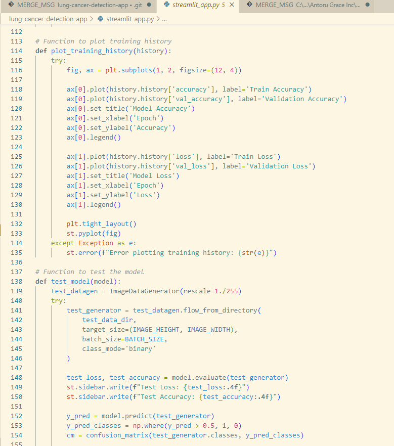
Snippet of my Streamlit application script on Vscode

 

4.2. Data

• Once the model coding has concluded, commence the next vital step: the data work.
• Select datasets that the CNN can manipulate from the data banks available on Kaggle, a renowned data science and machine learning platform, that featured CT scans either boasting cancer or images that were normal cases. Most of the information sets incorporate particular subtypes of lung cancer, such as large cell and squamous carcinoma, of which, as a side not, do not adversely affect the efficacy of the model, but rather equipping the model to better handle the various complexities it would subsequently encounter.
• The datasets of CT scans from Kaggle were the following: [26], [27], [28], [29]. The reasoning behind the use of four independent datasets essentially boils down to enriching the robustness and the generalization of the CNN, as exposure to a diverse range of data encourages the model to recognize new patterns instead of falling back on the memorization of a limited range of features. Despite that, only making use of four main datasets can be seen as a smaller quantity compared to the likes of Convolutional Neural Networks trained on over 15 000 distinct scans from numerous datasets, yet the significantly smaller quantity of four bodies of data can help the tackle the possible outcome of underfitting as well as efficiency and less computational magnitude, given the time available to train the model and finite storage of my computer.
• After the datasets are finally decided upon, download them unto an electronic device, preferably a computer, and create subfolders under a new folder, which is under an overall project CNN folder and environment responsible for story the information, scripts, Python environment and extensions of  the experiment, organizing the finds into separate directories containing the train, validation and testing assemblage, and properly labeling their contents.

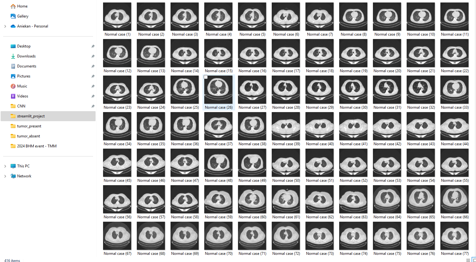
Example of the sub-folder hosting normal, non-cancerous CT scans

 

4.3. Merging Code and Data

• Develop a GitHub repository to store progress and scripts with the assistance of Git LFS, an extension of Git, or Google Drive, for files that surpass the 25 MB limit, in order for the app to recognize the directories of the dataset as well as the .keras file used to load the model, as both of the assets each take up more than 25 MB of storage.
• Be sure to not exceed the storage limit of 1 GB for Git LFS, or else the application will not work, and the system of the app will not be able to recognize the GitHub repository.
• Right now, the codes run locally, so in order for the scripts to be executed without the use of a command line shell, deploy the app after ensuring that all dependencies and environments from Python have been installed by creating a requirements text on GitHub responsible for housing all importations, and after composing all necessary files through the publication of the repository, as well as adding all additional files to the repository through:
  • Cloning the repository with the HTML handle.
  • Checking the status of the Git repository to identify any new changes that have not gone fully through into the repository.
  • Using the command 'git pull' to bring down any new commits that have not been accounted for.
  • Finally running the line 'git push' to the main repository.

Here is the link to the GitHub repository of my experiment: https://github.com/HeavenlyCloudz/lung-cancer-detection-app.git

 

4.4. Training and Evaluation

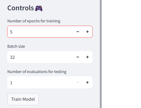
• After compiling the model and deploying the app, train the model on the data acquired, specifically deriving the training material from the subfolders of the data folder. Hopefully, the implemented app contains the appropriate functionalities and buttons to use to complete this process on the app itself instead of through some other obscure means.
• During the training of the model, record the accuracy and loss of the model in regard to the information of the training section, and equally record the accuracy and loss of the model in regard to the information of the validation section, detailing the results of the model to the data.
• Visualize the results of the training by plotting the model performance on a graph as well as plotting the confusion metrics of the testing performance of the model from the data (True Positive, False Positive, True Negative, False Negative, which in turn gives the information require for determining the F1 score, Precision, Overall Accuracy, and Recall)
• After every two days of the experiment, change the dataset to one of the 4 previously recommended in order to boost generalization and overall model performance.

Here is the link to the website of my model: https://readymag.website/u4174625345/5256774/

Even if everything is seemingly done correctly, expect an abundance of errors to arise and be prepared to be exposed to the world of debugging.

5. Observations

Everyday, I would record the results of my project, encompassing the outcome of the accuracy, loss, validation accuracy and validation loss, as well as other aspects of the given output I deemed to be significant. The following is the data that I have amassed:

Day	Results (Highest and lowest values out of the 20 epochs recorded)
1	32 steps/ epoch Epochs: 20 Accuracy: 1.0000, 0.9984                                Loss: 0.0000e+10, 11.0870                            Val-Accuracy: 0.9962                                                Val-Loss:  1.0174, 0.4470                            Notes: High accuracy and low loss might be an indicator of overfitting. Validation accuracy points to good generalization of the model on unseen data; validation loss could be improved. [26] Dataset: https://www.kaggle.com/datasets/adityamahimkar/iqothnccd-lung-cancer-dataset
2	32 steps/ epoch Epochs: 20 Accuracy: 1.0000, 0.7613 Loss: 0.0047, 10.9854 Val-Accuracy: 0.8675, 0.9255 Val-Loss: 0.6785, 2.0005 Notes: Similar results to the first day, but slightly lower in comparison. I wonder what the main factor in that might be. I equally noticed the model has significantly lower optimizer parameters than before, as well as parameters in general. Day 1 was still being done locally, without the deployment of the app and the introduction to Git Hub, so I assume that this is why the model was able to flourish and perform better than how it is currently performing, as I thought the results would improve and only become stronger, instead of becoming lower. The results of my data today still prove to be strong, but disappointing compared to the results of yesterday. However, it could be a positive sign, as the model is no longer overfitting the data and memorising but building those stronger connections. [26] Dataset: https://www.kaggle.com/datasets/adityamahimkar/iqothnccd-lung-cancer-dataset
3	32 steps/ epoch Epochs: 20 Accuracy: 1.0000, 0.6351 Loss: 0.0073, 6.9016e-05 Val-Accuracy: 0.8438, 0.7188 Val-Loss: 0.8933, 12.8460 Notes: Today was the day I switched datasets for the first time, so it would not be a far-fetched idea to believe the model initially had trouble adapting to the dataset, resulting in such a low score of 0.6351 to start. One would think that as the experiment progresses, the rate of accuracy would increase, but instead it seems like it is the opposite. I believe this argument can easily be excused by the switch in data, as the model stayed predominantly around 0.8000 - 0.9000. [27] Dataset: https://www.kaggle.com/datasets/borhanitrash/lung-cancer-ct-scan-dataset
4	32 steps/ epoch Epochs: 20 Accuracy: 0.5729, 1.0000 Loss: 0.0083, 2.9284e-04 Val-Accuracy: 0.7188, 0.9375 Val-Loss: 0.6397, 15.9307 Notes: My storage for the Git LFS is almost at capacity, which is probably impacting the performance of the model, as this is the first time the model has scored consistently lower than 0.6000 at any time during training, and a quick google search affirmed my suspicions. Thankfully, the model has been able to predict the class of the dataset at a percentage of 100% at least twice, which is an ideal score, however I tried to increase the performance of my model by introducing early stopping and using the transfer learning model MobileNetV3, but the default I wrote in my code was 'yes', and that default accidently sprouted some errors and added to the slowing down of the website, as well as the model lowering accuracy. [27] Dataset: https://www.kaggle.com/datasets/borhanitrash/lung-cancer-ct-scan-dataset
5	32 steps/ epoch Epochs: 5 (x4) Accuracy: 0.5599, 1.0000 Loss: 0.0143, 12.4574 Val-Accuracy: 0.2188,  0.8438 Val-Loss: 0.7585, 15.4882 Notes: I believe the results are lower than before because I didn't do all my epochs all together ( I did 5 epochs, and following those five, I did three more 5, instead of doing 20 epochs all together). Also, today was when I changed the contents of the dataset, so it is probably a bigger factor to the results of the model, as well as the continuous use of MobileNetV3. My storage is almost full, and I was afraid this was going to happen, provoking me to limit the number of epochs for training each day to 5 in order to not exhaust my available storage. Initially, I tried Google Drive, but it did not work well, however I believe that it is my last resort at my current state. I now understand it failed to work because I did not have the appropriate tools to make my data and model available on the Cloud and free to access. [28] Dataset: https://www.kaggle.com/datasets/subhajeetdas/iq-othnccd-lung-cancer-dataset-augmented?resource=download
6	32 steps/ epoch Epochs: 5 (x4) Accuracy: 0.6562, 1.0000 Loss: 0.1044, 0.9133 Val-Accuracy: 0.4545, 0.9845 Val-Loss: 0.2905, 0.3755 Notes: Today my Git LFS extension finally ran out of GB to accommodate to my model, so I am now using Git LFS + to store the .keras file of my model and the data of my model. Today, I equally implemented the EfficientNetB0 model, in order to speed up the process of learning, after first trying DenseNet121. Unfortunately, DenseNet121 was too heavy for my Streamlit application, and may have lowered results. The results of the data today were promising, as the EfficientNetB0 was already showing a glimpse of the competencies it possesses, giving me hope for an ideal outcome. [28] Dataset: https://www.kaggle.com/datasets/subhajeetdas/iq-othnccd-lung-cancer-dataset-augmented?resource=download
7	32 steps/ epoch Epochs: 5 (x4) Accuracy: 0.8259, 1.0000 Loss: 0.2970, 2.4095 Val-Accuracy: 0.8583, 0.9945 Val-Loss: 0.1275, 1.0259 Test- Accuracy: 0.9034, 1.0000 Test-Loss: 0.1026, 1.7289 Notes: Today was the first time I incorporated testing into the metrics of evaluation, and it acted as one of the determinants of the accuracy of my model. I introduced a new measure called confused metrics to quantify the F1 score, the recall, the precision and the overall accuracy. It is based off of the system of true positives, true negatives, false positives and false negatives, all used in order to determine the performance of ONCO AI. The results of my data today answered the paramount question of my experiment - if CNNs can classify lung cancer at an accuracy of 80% in one week, and the answer that I concluded from the experiment is yes. [29] Dataset: https://www.kaggle.com/datasets/mohamedhanyyy/chest-ctscan-images

6. Analysis

My custom CNN model, ONCO AI, was able to attain an incredible overall accuracy score of 80%, displaying the phenomenal proficiencies of CNNs in our time and age, and proving the verity of my proposed hypothesis. My model consistently reached and surpassed the target of 80%, exceeding my initial assumptions of the capacities of a CNN in the span of one week, with the following approximated result:

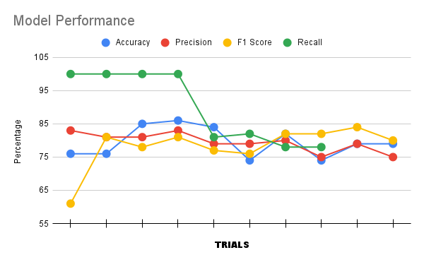
Graph of Final Day Model Testing

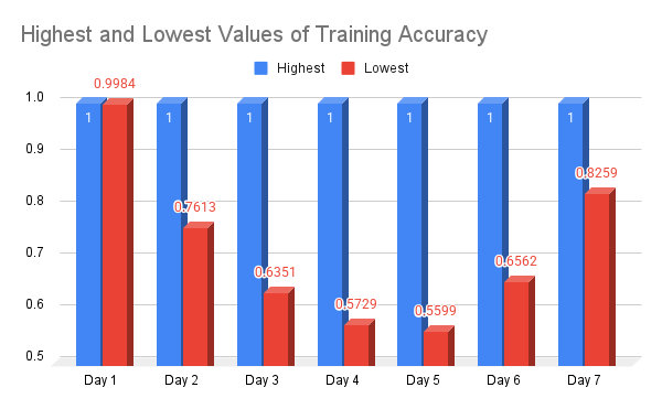
Graph of Daily Accuracy Observations

I experimented with various CNN architectures, such as the basic 3 convolutional layer CNN structure, MobileNetV3, Densenet121 and finally the EfficientNetB0 model, which produced the most rewarding results of all the frameworks tried. I recorded the results of all the models in addition to the EfficientNetB0 model to compare and contrast results. Initially, the model started off very strong, with high accuracy rates, but as the days of the experiment went on and the datasets evolved, the performance of my model slightly dipped, and I researched strategies to improve model performance in order to reach my end target of a 80% accuracy, including the utilization of Adam in particular as my optimizer of choice, yielding a quicker learning rate, and the utilization of transfer learning, an appealing method to exposing the model to a wider variety of data types. In the beginning, I started at 20 epochs per training session, and the performance of my application was not affected. However, as the resource limit of my Streamlit app was met, error would continuously plague my software, hindering me from effectively using ONCO AI. Thankfully, I found a cost-effective approach that greatly reduced my daily resource intake on Streamlit once I set my epochs on the app for training to a seemingly inadequate, yet advantageous 5, defining the number of times my CNN goes through my entire dataset.

 

6.1. Considerations

During the course of my experiment, I found the project to be primarily built around the art of debugging. The code and wiring of my programs endured countless changes and refinements in order for the model to function smoothly, without flaw or error. It seemed as if the correction of one blunder fed directly into the creation of a new oversight, and the maddening process prevailed time and time again, even when I determined my script to be good. Initially, the model refused to display the output of the prediction through the means of the Grad CAM, as a recurring error concerning the lack of initialization of the layer Sequential prohibited the code from doing so. 

Another important factor of my experiment was the determining of which transfer learning model to use, and which ones worked best for my current circumstances. Here are the metrics that influenced the decision of my final model design:

Models

Metrics	Traditional	MobileNetV3	DenseNet121	EfficientNetB0
Accuracy	1.000, 0.5345	0.6738, 0.4897	0.7984, 0.4834	1.0000, 0.6562
Loss	11.0870 ,0.0000e+10	0.0527, 0.0158	0.9133, 0.2487	0.9549, 0.2479
Val-Accuracy	0.9962, 0.6921	0.9375, 0.2188	0.9845, 0.4975	0.9945, 0.7545
Val-Loss	12.8400, 0.0047	15.9307, 0.6397	0.7895, 0.1275	1.0259, 0.1275

 

Ultimately, I continued with EfficientNetB0 as the concluding transfer model of my experiment, and I consider it a well-founded decision.

 

7. Conclusion

CNNs are powerful devices that are able to learn at an extremely fast rate when given the appropriate resources to succeed. ONCO AI provides an exemplary demonstration of the capabilities these neural networks can possess, as the CNN has a high detection accuracy rate with the potential of progressing further. Their implementation alongside other medical diagnosis tools could greatly reduce the massive impact of lung cancer, ensuring one of the most vital organs of our bodies is protected from the severity of lung cancer early on. My primary objective is that through this fair, and online promotion, this experiment will inspire others to delve deeper into the electrifying world of deep neural networks, specifically CNNs, propelling the closure of the information and availability gap for those affected or equally interested in cancer. There is still a long way to go to ensure that the CNN is fully equipped to consistently understand the scans that it is presented with, as well as generating predictions that are true, but based on the current design of ONCO AI, the algorithm is a trustworthy CNN, given the time it had to learn patterns in the data it was shown.

The front-end page of ONCO AI with information about the experiment

8. Application

My experiment conducted on the abilities of CNNS has real-world implications, as progress and future development of deep learning algorithms in medical research regarding cancer, and other forms of illnesses leads us as a society one step closer in the objective of introducing quality solutions to slowly eradicate the severity of the disease. The study of cancer and novel solutions that artificial intelligence continues to formulate are extremely promising, considering the significant advances of just the last few years with the creation of copious medical analysis chatbots and other neural networks built to care to the needs of patients, as well as to the regular demands of everyday life. Nevertheless, the funding of lung cancer research in Canada is inadequate compared to the likes of other major types of cancer [2], therefore the persistent application of Convolutional Neural Networks working alongside professionals to better comprehend lung cancer and probable solutions to combat the cancer will not only positively impact the field of lung cancer research, but it will equally improve the quality of life for millions of patients globally and greatly influence the direction of synthetic intelligence among other fields in the medical community, embracing the leveraging of powerful automated tools to save the lives of many. However, I personally believe the ethics of neural networks begins to become murky once the notion that AI supersedes the existence of radiologist and the various domains that intertwine with the abilities of deep learning networks is brought into discussion, as the models should not be the primary basis, or source of truth. That assumption should always rest on the professional who attended rigorous training to attain the position they currently possess. Unfortunately, current progress of artificial intelligence is posing a threat to certain critical fields that are deemed as being roles synthetic intelligence could easily replace, specifically artistic disciplines, and even certain radiology occupations, given the fact that some models have already demonstrated their superiority to radiologists in their predictions of cancer. Several researchers of cancer debate of the topic of full artificial intelligence implementation into healthcare, and discourse is divided about the full extent deep neural network programs, such as CNNs, can be integrated into the medical imaging sphere in years to come.

9. Sources of Error

Potential blunders executed on my part that may have negatively impacted the outcome of my experiment, encompassing the reliability and precision of my CNN, ONCO AI, was the slowly diminishing number of epochs that I completed during the training process. Traditional starting points for epochs during training is anywhere between 50-100 (Google Search), and unfortunately, I was unable to follow this format given the fact that several storage constraints perpetuated by the Streamlit program and my GPU prohibited my CNN from consuming an overabundance of memory while training. This limited the number of epochs down to only 5 during the last few days of my experiment, far from the recommended 50 of my quick, surface-level Google inquiry. However, I managed to combat the lower epochs with a higher batch rate of 32-64, and I employed a strategy known as transfer learning, where I implemented a pre-built CNN structure into my overall CNN code to counter the lack of adequate epochs and weight improvement that had initially confronted me.

Moreover, my algorithm held a bias towards cancerous images, as images that were cancerous were far larger than those of the contrary among the datasets I required, resulting in the outcomes of the matrix displaying the fact that false positives had a stronger presence than false negatives due to their oversaturation.

On day 5, the change of my dataset initially seemed to go smoothly, but there were images among the inventory of collected data that were incorrectly labeled, conceivably leading to fluctuations and decrease in the training and validation accuracy of ONCO AI.

Furthermore, limited computational resources, such as memory, storage and GPU restricted the continuous use of more avant-garde transfer learning frameworks, such as the likes of Densenet121, VGGNet-16, or ResNet, as my Streamlit application did not possess the disk space required to run these models, restraining hyperparameter tuning diversity that should have been accessible to the CNN. Fortunately, I was able to counter this downside with a transfer learning model that light-weight model that has a high accuracy rate in EfficientNetB0.

One last substantial error is the fact that there were a handful of CT scans that might have been ambiguous, feasibly belonging to either class, especially for a model during the training phase, potentially hindering the model from developing strong connections necessary to differentiate between cancerous and non-cancerous CT scans.

9.1. Room for Improvement

For future considerations of this experiment, I will use the Pro version of Streamlit, or another heavy model-friendly open-source Python framework, in the hope of supplying my model the imperative space to function without being limited to the confines of an insufficient asset quantity, just as how I upgraded my Git LFS to accommodate increased file sizes via extended storage. However, I would have to reassess the budget of my experiment to adapt to the elevated cost from these acquisitions. Following this approach, I would not be forced to endure the bounded epoch window for training and validation, broadening the scope of epoch range and equally accelerating learning speed.

In order to tackle the problem of bias in the network, I will oversaturate the minority class of non-cancerous images so as to mitigate class bias in the model, as the datasets I found had a higher ratio of cancerous CT scans to non-cancerous CT scans. Due to my limited time, and prioritization of code debugging, my focus ignored the finer details of the data, resulting in the reduced attention of class proportion. Next time, I would be more proficient in coding, and troubleshooting would not be a top-priority during the course of the experiment.

LUNG CANCER:

[1] Functions of blood: transport around the body (n.d.).  blood.co.uk - https://www.blood.co.uk/news-and-campaigns/the-donor/latest-stories/functions-of-blood-transport-around-the-body/#:~:text=Haemoglobin%20molecules%20inside%20red%20blood,for%20the%20transport%20of%20oxygen.

[2] Facts about Lung Cancer (n.d.). lungcancercanada.ca - https://lungcancercanada.ca/about-lung-cancer/facts-about-lung-cancer/#:~:text=About%20Lung%20Cancer-,Today%2C%20lung%20cancer%20remains%20the%20most%20commonly%20diagnosed%20cancer%20in,prostate%20and%20colon%20cancer%20combined.

[3] Lung Cancer Guide | What You Need to Know (n.d.). cancerguide.org - https://www.cancer.org/cancer/types/lung-cancer.html

[4] Lung Cancer Types, Stages, Symptoms, Diagnosis & Treatment (10/31/2022). myclevelandclinic.org - https://my.clevelandclinic.org/health/diseases/4375-lung-cancer 

[5]  Lung cancer (06/23/2023). who.int - https://www.who.int/news-room/fact-sheets/detail/lung-cancer

[6] Manage Shortness of Breath with Lung Cancer (n.d.). hopkinsmedicine.org - https://www.hopkinsmedicine.org/health/conditions-and-diseases/lung-cancer/manage-shortness-of-breath-with-lung-cancer#:~:text=Blocked%20airways%3A%20Lung%20tumors%20can,wall%2C%20called%20the%20pleural%20space.

[7] Computed Tomography (CT) (n.d.). nibib.nih.gov - https://www.nibib.nih.gov/science-education/science-topics/computed-tomography-ct

[8] What Does Lung Cancer Look Like? (07/10/2024). Lindsay Modglin. patientpower.info - https://www.patientpower.info/lung-cancer/what-does-lung-cancer-look-like

 

DEEP LEARNING (CNNS + APP CODE):

[9] Convolutional neural networks in medical image understanding: a survey (01/03/2021). D R Sarvamangala ¹, Raghavendra V Kulkarni ².  pmc.ncbi.nlm.nih.gov - https://pmc.ncbi.nlm.nih.gov/articles/PMC7778711/

[10] Neural Networks and Deep Learning (Last Updated: [12/26/2019]). Michael Nielsen. neuralnetworksanddeeplearning.com - http://neuralnetworksanddeeplearning.com/index.html

[11] Hands-On Deep Learning Algorithms with Python (July 2019). Sudharsan Ravichandiran - https://www.google.ca/books/edition/Hands_On_Deep_Learning_Algorithms_with_P/8DqlDwAAQBAJ?hl=en&gbpv=1&pg=PP2&printsec=frontcover

[12] Hands-On Machine Learning with Scikit-Learn, Keras, and Tensorflow (03/13/2017).  Aurelien Geron -  https://www.google.ca/books/edition/Hands_On_Machine_Learning_with_Scikit_Le/HnetDwAAQBAJ?hl=en&gbpv=1&pg=PT3&printsec=frontcover

[13] The Role of Geometry in Convolutional Neural Networks for Medical Imaging (09/30/2023). Yashbir Singh M.Tech, PhD ^a, Colleen Farrelly MS ^c, Quincy A. Hathaway MD, PhD ^d, Ashok Choudhary PhD ^b, Gunnar Carlsson PhD ^e, Bradley Erickson MD, PhD ^a, Tim Leiner MD, PhD ^a. sciencedirect.com - https://www.sciencedirect.com/science/article/pii/S2949761223000743#:~:text=This%20hierarchical%20representation%20enables%20CNNs,such%20as%20tumors%20or%20lesions

[14] Convolutional neural network (June 2019). en.wikipedia.org - https://en.wikipedia.org/wiki/Convolutional_neural_network

[15] Exploring Convolutional Neural Networks: Architecture, Steps, Use Cases, and Pros and Cons (04/24/2023). Tamanna. medium.com - https://medium.com/@tam.tamanna18/exploring-convolutional-neural-networks-architecture-steps-use-cases-and-pros-and-cons-b0d3b7d46c71

[16] Perceptron vs neuron, Single layer Perceptron and Multi Layer Perceptron (09/21/2024). Abhishek Jain. medium.com - https://medium.com/@abhishekjainindore24/perceptron-vs-neuron-single-layer-perceptron-and-multi-layer-perceptron-68ce4e8db5ea#:~:text=A%20neuron%2C%20or%20artificial%20neuron,can%20have%20multiple%20hidden%20layers

[17] Understanding binary cross-entropy / log loss: a visual explanation (11/21/2018). Daniel Godoy. towardsdatascience.com - https://towardsdatascience.com/understanding-binary-cross-entropy-log-loss-a-visual-explanation-a3ac6025181a/

[18] Introduction to Deep Learning (08/02/2023). Tommy Kim. velog.io - https://velog.io/@ktm1237/MIT-Introduction-to-Deep-Learning

[19] Create an app - Streamlit Docs (n.d.). docs.streamlit.io - https://docs.streamlit.io/get-started/tutorials/create-an-app

[20] Convolutional Neural Network (CNN) (n.d.). tensorflow.org - https://www.tensorflow.org/tutorials/images/cnn

[21] Understand the Grad-CAM: A Complete Guide With Example (09/21/2023). codetrade.io - https://www.codetrade.io/blog/grad-cam-a-complete-guide-with-example/

[22] Convolutional Neural Networks: A Brief History of their Evolution (08/31/2021). medium.com - https://medium.com/appyhigh-technology-blog/convolutional-neural-networks-a-brief-history-of-their-evolution-ee3405568597

[23] Neuron (n.d.). en.wikipedia.org - https://en.wikipedia.org/wiki/Neuron

[24] Difference between Empirical Loss and Expected loss (Modified 2 years, 11 months ago). math.stackexchange.com - https://math.stackexchange.com/questions/4426769/difference-between-empirical-loss-and-expected-loss

[25] Xavier and He Normal (He-et-al) Initialization (09/29/2018). Vishnu Kakaraparthi. prateekvishnu.medium.com - https://prateekvishnu.medium.com/xavier-and-he-normal-he-et-al-initialization-8e3d7a087528

 

IMAGING:

[26] IQ-OTH/NCCD - Lung Cancer Dataset (2021). Aditya Mahimkar. kaggle.com - https://www.kaggle.com/datasets/adityamahimkar/iqothnccd-lung-cancer-dataset

[27] Lung Cancer CT Scan Dataset (Updated 8 months ago). Md. Abdur Rahman. kaggle.com - https://www.kaggle.com/datasets/borhanitrash/lung-cancer-ct-scan-dataset

[28] IQ-OTH/NCCD Lung Cancer Dataset (Augmented) (Updated a month ago). Subhajeet Das. kaggle.com -

https://www.kaggle.com/datasets/subhajeetdas/iq-othnccd-lung-cancer-dataset-augmented?resource=download

[29] Chest CT-Scan images Dataset (Updated 5 years ago). Mohamed Hany. kaggle.com - https://www.kaggle.com/datasets/mohamedhanyyy/chest-ctscan-images

 

IMAGE CREDITS:

Figure 1.3.1: Lung Cancer CT Screening (n.d.). sd.imaging.com - https://www.sdimaging.com/lung-scan/

Figure 1.4.1: An Easy Guide to Neuron Anatomy with Diagrams (Updated 02/28/2022). Medically reviewed by Nancy Hammond, M.D. — Written by Carly Vandergriendt and Rachael Zimlich, RN, BSN. healthline.com - https://www.healthline.com/health/neurons

Figure 1.4.1.1: Sigmoid Activation Function: An Introduction (07/10/2023). Noah Topper. builtin.com - https://builtin.com/machine-learning/sigmoid-activation-function

Figure 1.4.1.2: Sigmoid function (n.d.). en.wikipedia.org - https://en.wikipedia.org/wiki/Sigmoid_function

Figure 1.4.1.3: 1a. The Unit Step Function (Heaviside Function) (n.d.). www.intmath.com - https://www.intmath.com/laplace-transformation/1a-unit-step-functions-definition.php

Figure 1.5.1: Introduction to Deep Learning (08/02/2023). Tommy Kim. velog.io - https://velog.io/@ktm1237/MIT-Introduction-to-Deep-Learning

Figure 1.5.2: Binary Cross Entropy: Where To Use Log Loss In Model Monitoring (01/01/2023). Amber Roberts. arize.com - https://arize.com/blog-course/binary-cross-entropy-log-loss/

Figure 1.6.1: Introduction to Deep Learning (08/02/2023). Tommy Kim. velog.io - https://velog.io/@ktm1237/MIT-Introduction-to-Deep-Learning

Figure 1.6.2: Weight initialization (05/17/2021). Uomnf97. velog.io - https://velog-io.translate.goog/@uonmf97/Weight-initialization?_x_tr_sl=auto&_x_tr_tl=en&_x_tr_hl=en&_x_tr_pto=wapp

Figure 1.6.3:  Introduction to Deep Learning (08/02/2023). Tommy Kim. velog.io - https://velog.io/@ktm1237/MIT-Introduction-to-Deep-Learning

Figure 1.7.1:  Introduction to Deep Learning (08/02/2023). Tommy Kim. velog.io - https://velog.io/@ktm1237/MIT-Introduction-to-Deep-Learning

Figure 1.7.2:  Introduction to Deep Learning (08/02/2023). Tommy Kim. velog.io - https://velog.io/@ktm1237/MIT-Introduction-to-Deep-Learning

Figure 2.1.1.1: The Probabilistic Origin of Regularization (08/19/2023). Avi Chawla. dailydoseofds.com - https://www.dailydoseofds.com/the-origin-of-regularization/

Figure 2.3.1: Convolutional Neural Networks (08/29/2023). Tommy Kim. velog.io - https://velog.io/@ktm1237/Convolutional-Neural-Networks#computer-vision

Figure 2.3.2: Convolutional Neural Networks (08/29/2023). Tommy Kim. velog.io - https://velog.io/@ktm1237/Convolutional-Neural-Networks#computer-vision

Figure 2.5.1: CNN | Introduction to Pooling Layer (Last Updated: 02/04/2025). geeksforgeeks.org - https://www.geeksforgeeks.org/cnn-introduction-to-pooling-layer/

 

 

 

I would like to express my immense gratitude to all those who have contributed their time to assist me on this challenging, yet wonderful expedition on the exploration and application of Convolutional Neural Networks to identify lung cancer. To begin, I want to extend my appreciation to my incredible parents, Dr. Aniekan Udofia and Williams Udofia, who took thier time to review the written portion of my work; pushed me to my limit even when I felt the project was beyond me; and gave me indispensable insight on the fascinating world of coding, sharing captivating articles and resources that aided in the creation and implementation of my neural network respectively. I would additionally like to share my gratitude to my Grade 9 Science teacher, Mme. Scholz, for reviewing the beginning drafts of my project, suggesting important commentary on aspects of my writing that were lacking, and equally providing the opportunity for me to attend the Calgary Youth Science Fair.