1.0 Abstract

The origins of the universe are a mystery many are working to uncover. Molecular clouds are a key part of this mystery. Molecular clouds have the nickname of 'solar nurseries' due to being the birthplace of stars and planets. If humans can better understand how molecular clouds form, where they form, and what they are composed of, we can then better understand our universe. This research is intended to prove the hypothesis that by looking at a large number of star forming regions you can infer how diverse they really are. Through the utilisation of Machine Learning algorithms it was concluded that molecular clouds do not have distinct clusters, meaning that they are are capable of creating similar life forms. This was concluded due to the failure of clustering algorithms such as Gaussian Mixture Models and Kmeans Clustering to produce convincing clusters with appropriate Davies Bouldin and Silhouette Scores. Furthermore, it can be concluded that most features do not have a large effect on CO emissions from molecular clouds due to the low R-squared scores, and large Mean Absolute Error scores produced by supervised regressions algorithms such as Linear Regression, Kmeans Regressor, and the AdaBoot Regressor amongst others. The low diversity of planetary forming regions may mean that it is likely for more habitable planets to be produced from any molecular cloud.

1.1 Problem Statement and Hypothesis

This paper is intended to prove that by looking at a large number of star forming regions, or molecular clouds, you can infer how diverse molecular clouds in the milky way galaxy really are.

2.0 Method

2.1 Methodology

This paper utilised a continuous dataset due to the nature of this topic. The dataset is not split into categories as molecular clouds are only grouped based on mass which is a continuous measure. The dataset utilised is from the National Aeronautics and Space Administration most commonly referred to as NASA.

2.2 Understanding Machine Learning

2.2.1 Data Cleaning

Typically for code, regardless of the language, you must start with imports. Imports are essentially lines of codes that connect to other 'libraries' or collections of code that make coding simpler and neater. For machine learning some necessary libraries are numpy, pandas, sklearn, and matplotlib. Numpy is one of the most common coding libraries and is used for operations and computing. Pandas, another important library, aids in cleaning and manipulation of data. Matplotlib is used for data visualisation and graphing Finally, sklearn is the main library which contains the machine learning algorithms utilised within this paper. Typically the pandas algorithm is shortened to pd as it will often be used. The numpy algorithm is shortened to np, and the matplotlib library is shortened to plt. See Figure 1 for the imports of the library used. Note that seaborn is commented out (not affecting the code) due to it causing errors, though it is often included due to its close integration with pandas and matplotlib. Furthermore, other libraries will be imported later on in the code as they become necessary.

Figure 1: Imports of pandas, numpy, matplotlib, and sklearn libraries 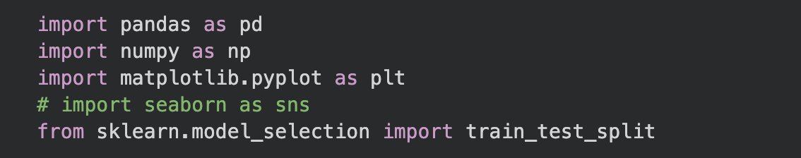Line one is the pandas import, with the as keyword allowing the coder to reference pandas and call it later on in the code through the shorter 'pd' rather than pandas. Line two is the import of numpy with the as keyword shortening it to np. Line three is the import of matplotlib shortening it to plt. Line four is commented out due to the hashtag and green colour, meaning that it does not affect the code. Finally line five is the Sklearn import.

It is crucial to import the dataset that will be analysed. This requires the dataset to be downloaded as a csv or a comma separated value. The dataset is downloaded as "table1_full - table1_full.csv" on the computer. Therefore to reference the dataset it must be written with exactly the same notation. Through pandas the name of the dataset can be changed to df, and it can be represented as a table. See Figure 2.

Figure 2: Adding the dataset to the code 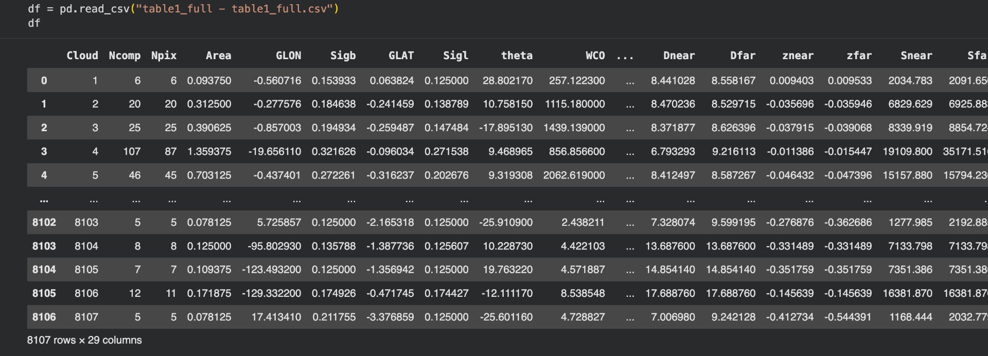Line one allows the dataset to be referred to as df, and line two prints it out. Note that the dataset cuts off in the picture as Sfar, but it goes further in the actual code. Furthermore, in many code languages and IDEs df alone would not print, but collab notebook (where this code is being written) has a unique function where printing the name of a variable prints it out.

Finally, for data cleaning you need to remove NaNs (Not a number) or places where the information was not properly filled out causing issues for the code. This can be done by deleting unnecessary columns and rows. For this dataset there are no NaNs to be deleted. Theoretically many columns were unnecessary as they were not utilised later in the code. The only column truly useless was Cloud Number as the rows were automatically given numbers eliminating that columns use. Note that whenever df is mentioned in the future it means dataframe. See Figure 3.

Figure 3: Removing Unnecessary Columns 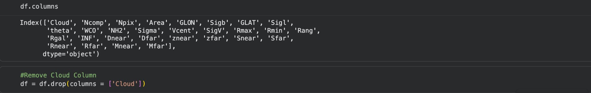df.columns simply prints all of the column titles. df = df.drop(columns = ['Cloud']), deleted the column 'Cloud' and updated df to represent the deleted version.

2.2.2 Basic Representation

This section utilises scatterplots. Note that in the actual code histograms were created. However, because they were not essential to the study all of the histograms, and several of the scatterplots will not be discussed. If you wish to see those plots you are more than welcome to use this link: https://colab.research.google.com/drive/1Qt_Jau4zjK3GH3DpVur_mywLBqJJIQcz#scrollTo=eNWwnvf8B3To. For the data representation, and the rest of this paper you must understand what some of the key features are and what they mean. Features are the columns or the individual variables of the dataset. The most important feature is WCO, or Integrated carbon monoxide emission, as mentioned later in the research. See Figure 4 below for the feature guide. Note that within the code features S, N, R, D, and Z will be referred to as Snear, Near, Rnear, Dnear, and Znear which represents the nearest estimate.

Figure 4: Feature Guide 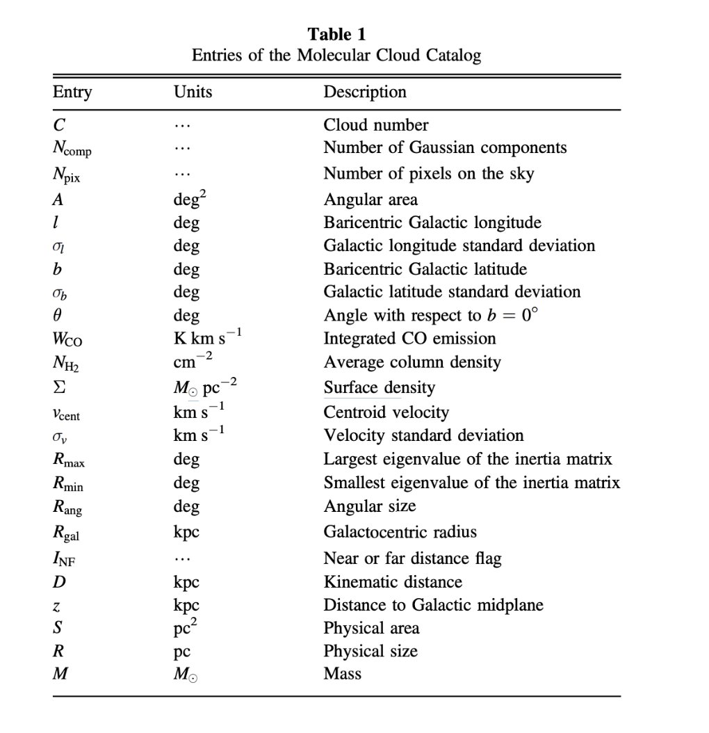A guide containing all the features within the dataset.

Scatterplots are a way to represent continuous data. They use dots to represent where each data point is on each axis. When analysing large datasets it is important to utilise logarithms to properly assess the scale of the data. Some metrics such as Mnear range from 10^-2 to 10^6, which is from 0.01 to 1,000,000. Logarithms allow for this range to be properly represented. See figure 5.

Figure 5: WCO vs Mnear Scatterplot 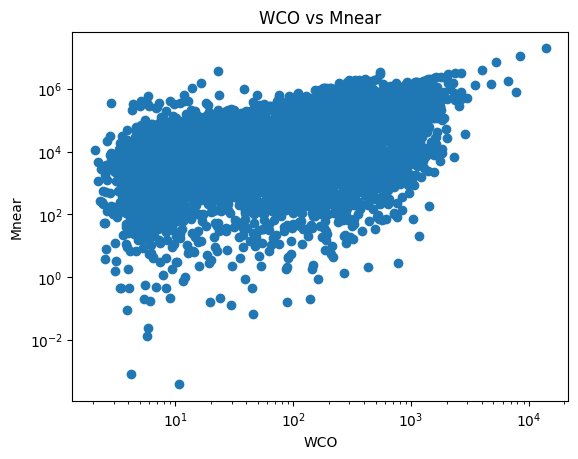A scatterplot that shows WCO compared to the wide range of Mnear from 10^-2 to 10^6.

2.2.3 Unsupervised Learning

For unsupervised learning two clustering algorithms were utilised; these were Kmeans Clustering and Gaussian Mixture Models (GMM). Essentially they attempt to find various parts of the graphs, or distinct clusters. These are analysed by Davies Bouldin and Silhouette scores which come from the sklearn library.

Kmeans clustering requires a set amount of clusters to find and look for, as does GMM clustering. The number of clusters is determined through what is essentially brute force. The code runs through various numbers of clusters and runs an analysis using Davies Bouldin and Silhouette Scores which determine which number of clusters performed the best. Kmeans clustering can be greatly affected by outliers, and can't properly model all patterns. Also, it does not perform well in uneven clusters. The quality of the results highly depends on the clusters being split into distinct groups.

Figure 6: WCO vs Sigma Kmeans Clustering Kmeans clustering fails to produce a convincing result.

GMM clustering is known as the best alternative to Kmeans clustering. GMM stands for Gaussian Mixture Models. The name implies Gaussian Mixture Models allow points to be in a 'mixture' of clusters, and is 'softer' compared to Kmeans as it assigns probabilities to each point being within a cluster. Gaussian Mixture Models were used together with Kmeans clustering to try and get better results. See figure 7.

Figure 7: WCO vs Sigma GMM Clustering 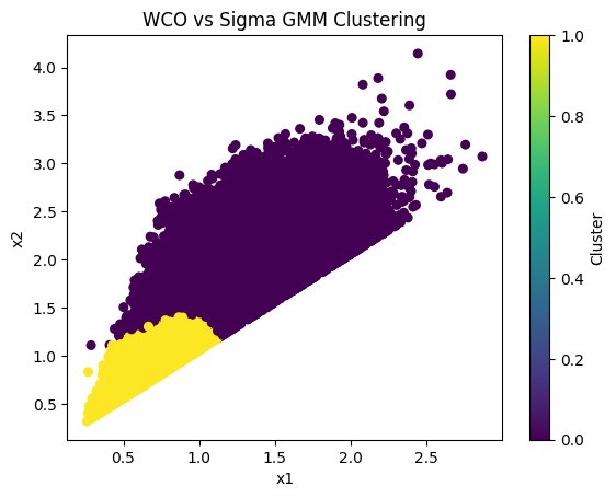The result of gaussian mixture models on the original WCO vs Sigma scatterplot, which failed to produce convincing results.

As mentioned earlier the Davies Bouldin Metric and the Silhouette Score metric are ways to analyse the effectiveness of the clustering. Davies Bouldin looks for clusters that are farther apart and have clear regions. The Silhouette Score metric calculates the distance between a point and its nearest cluster that it is not a part of (similar to how kmeans clustering works). Davies bouldin scores start at zero and the lower the score the better. A good silhouette score is +1, with the worst being -1.

2.2.4 Supervised Learning

Supervised learning algorithms include linear regression, MLP regressor, random forest regressor, and k-means regressor. Unlike unsupervised learning algorithms, supervised learning algorithms require a train-test split, to check the accuracy of the algorithm. The typical split is 80-20, with 80% being training, 20% being testing. See Figure 8.

Figure 8: Train-Test split and Assignment of X and y 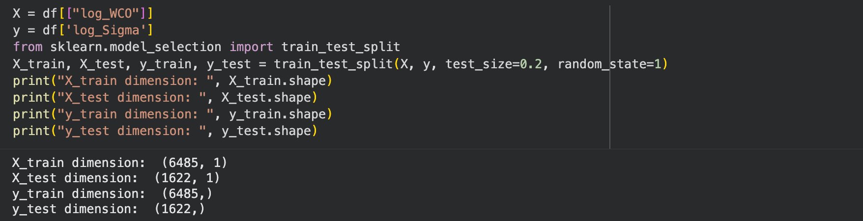Line four defines the training and testing split, with the print statements afterwards simply allows for an understanding of the size of the datasets to confirm I didn't make any mistakes. Note that in common convention 'X' is uppercase and 'y' is lowercase.

In order to utilise the algorithms they must be imported similarly to the imports at the beginning of the code. Most of the imports were only added as needed rather than all together. Once imported I started with the Random Forest Model, which is based on decision tree algorithms. Rather than using one decision tree, random forest utilises multiple. See Figure 9.

Figure 9: Imports and Random Forest 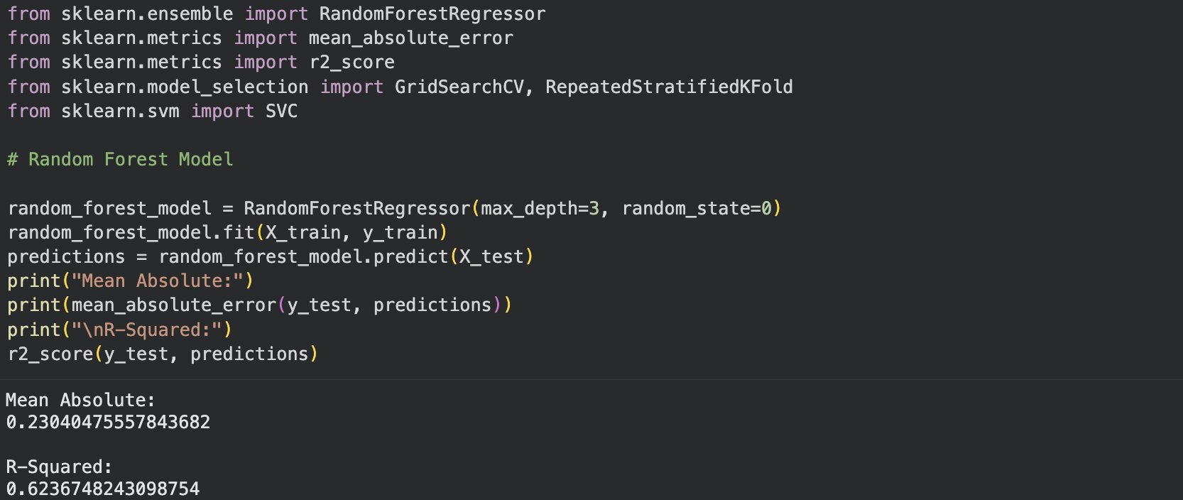The imports needed for the supervised learning and analysis as well as the Random Forest Model.

Hyper-parameter tuning allows for a machine learning model to have the maximum possible performance. This tunes the number of 'layers' utilised and prevents overfitting. The ideal shape is similar to the classic bell curve where the model's accuracy continues to rise until it drops. See figures 10 and 11.

Figure 10: Code for Hyper-parameter Tuning 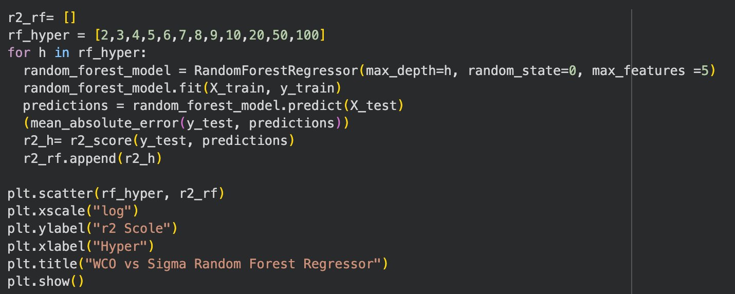The code utilised to conduct hyper-parameter tuning specifically on the Random Forest Regressor Model.

Figure 11: Visual representation of the Random Forest Regressor's Hyper-parameter tuning on the WCO vs Sigma graph Shows a curve starting at \~0.595 and increasing to \~0.62 before dropping. compares the hyper-parameter to the R^2 score.

The Adaboost, Linear Regression, MLP Regressor (Multi-Layer Perceptron Regressor), and KNeighbors Regressor were also utilised. They all produced similar results and therefore will not be explored in depth. The Mean Absolute Error scores and R^2 Scores as mentioned earlier are ways to analyse the effectiveness of the supervised learning algorithms. A good Mean Absolute Error score is close to zero, and a good R^2 Score is close to 1.0.

Finally, no classification algorithms were utilised due to the dataset being continuous and therefore not having categories to predict. Overfitting is a notable problem which can be reduced by having large amounts of training data, having a suitable train-test split, and through data cleaning.

3.0 Background Information

3.1 Understanding Molecular Clouds

Stars are formed in molecular clouds, which are essentially large dusty regions in space. To our current scientific understanding there are no types of molecular clouds in any way other than mass. The term GMC or Giant Molecular Clouds, refers to clouds around a density of 150cm-3 (Science Direct). Molecular clouds are the densest interstellar clouds and are also incredibly cold. They are mainly made of hydrogen (H2), as well as organic compounds. A key component of Molecular Clouds are carbon monoxide emissions which scientists use to trace molecular cloud structures. The Centre for Astrophysics Harvard and Smithsonian explains that stars are born in the densest and most opaque molecular clouds.

According to a paper by Shigenori Maryama et al. There are nine requirements for the formation of life. These are an energy source, a supply of nutrients, a supply of life-constituting major elements, a high concentration of reduced gases, dry-wet cycles, a non-toxic aqueous environment, Na-poor water, highly diversified environments, and cyclic conditions. The most important requirements in regards to this paper are a supply of life-constituting major events, and a high concentration of reduced gases. The six 'elements of life' are known as C.H.N.O.P.S. or carbon, hydrogen, nitrogen, oxygen, phosphorous, and sulfur (Remick and Helman).

Physical Properties of Molecular Clouds For The Entire Milky Way Galaxy is a 2017 paper by Marc-Antoine Miville-Deschênes et al. They go over the importance of surface density (represented as sigma) to molecular cloud formation. It agrees with my results of surface density and radius having little to no correlation. Surface Density (sigma) and Carbon Monoxide have a known correlation which is preprogrammed into the dataset.

Results: https://colab.research.google.com/drive/1Qt_Jau4zjK3GH3DpVur_mywLBqJJIQcz?usp=sharing

3.0 Data

Once again, note that to review all of the data collected click the results link above. This dataset is from NASA and was most recently updated January 2026.

WCO vs Sigma is perhaps the most important comparison of metrics in this paper. Sigma refers to the surface density of the molecular clouds. The scatterplot below represents WCO and Sigma in relation to each other. (See Figure 1) There is a clear linear relation between the surface density and integrated carbon monoxide emissions which was pre-programmed. Note that clustering algorithms but 'soft' and 'hard' fail to produce effective clusters within the dataspace.

Figure 12: WCO vs Sigma represented through a Scatterplot 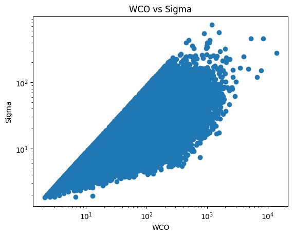WCO as mentioned earlier represents integrated carbon emissions and is the main feature analysed throughout this dataset. Sigma represents surface density of the molecular cloud. Both features are represented with the use of logarithms in order to properly represent the large range of data. The straight line is a preprogrammed relation.

Figure 13: WCO vs Sigma represented through a Scatterplot and Gaussian Mixture Model Clustering Unconvincing clustering produced by Gaussian Mixture Models on the WCO vs Sigma data-space, describing integrated carbon monoxide emissions in relation to surface density.

Figure 14 WCO vs Sigma Kmeans Clustering: 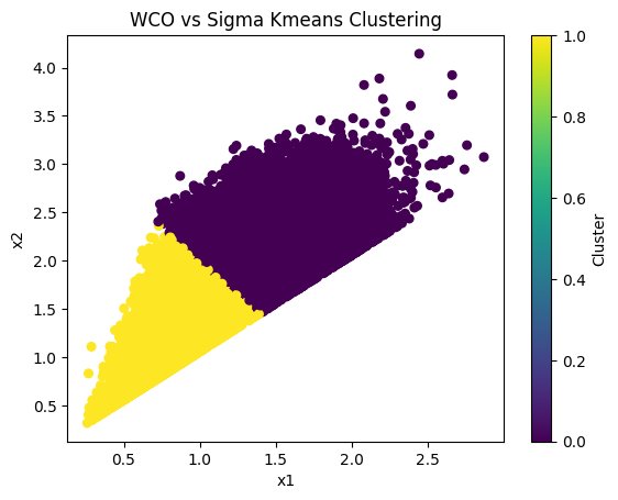Unconvincing clustering produced by the Kmeans Clustering Model on the WCO vs Sigma data-space, describing integrated carbon monoxide emissions in relation to surface density.

Figure 15: WCO vs Sigma Random Forest Regressor: 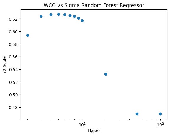A visual representation of the results of supervised regression using the Random Forest Regressor on the WCO vs Sigma data space, using R^2 scores. Shows the typical bell curve with the largest point being just above 0.62.

Figure 16: WCO vs Sigma Linear Regression Model with R-squared and Mean-absolute-error scores 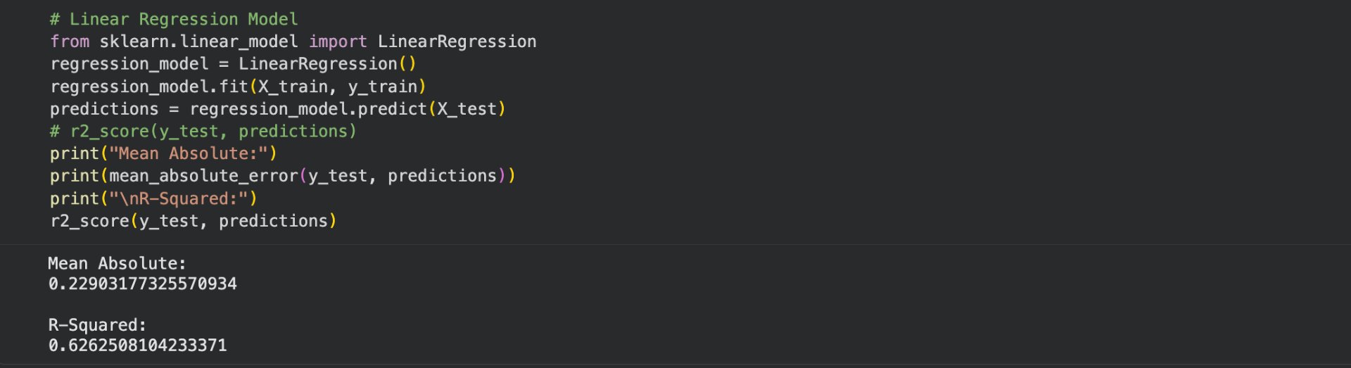The resulting mean absolute error and R^2 scores of the data space using linear regression. The mean absolute error score being \~0.22, and the R^2 score being \~0.63, both respectable scores, showing an existing correlation.

Figure 17: WCO vs Snear represented through a Scatterplot 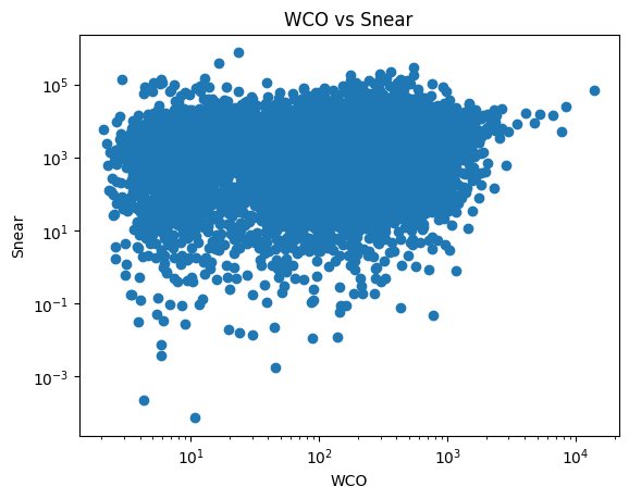A representation of integrated carbon emissions in relation to the nearest estimate of physical area of the respective clouds. Utilises logarithms for proper representation of the dataset.

Figure 18: WCO vs Snear Gaussian Mixture Model Clustering 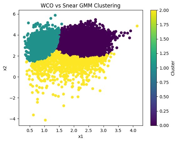Unconvincing clusteing produced by Gaussian Mixture Models on the WCO vs Snear dataspace.

Figure 19: WCO vs Snear Kmeans Clustering: 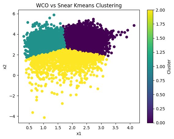Unconvincing clusteing produced by the Kmeans Clustering Model on the WCO vs Snear dataspace.

Figure 20: WCO vs Snear Random Forest Regressor: 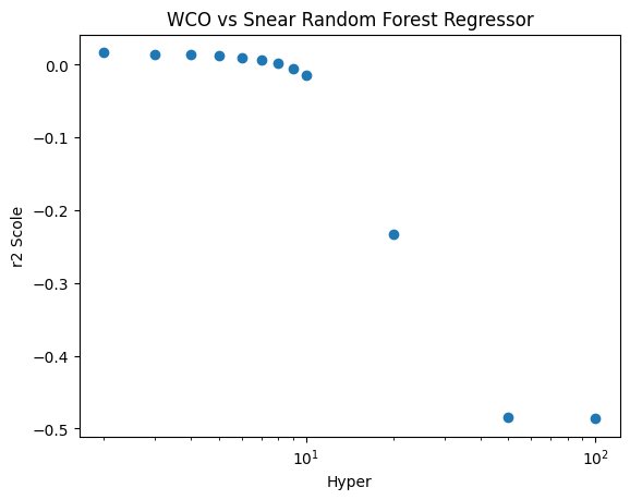A visual representation of the resuls of supervised regression using the Random Forest Regressor on the WCO vs Snear data space, using R^2 scores. Shows absolutely no relation.

Figure 21: WCO vs Snear Linear Regression Model with R-squared and Mean-absolute-error scores 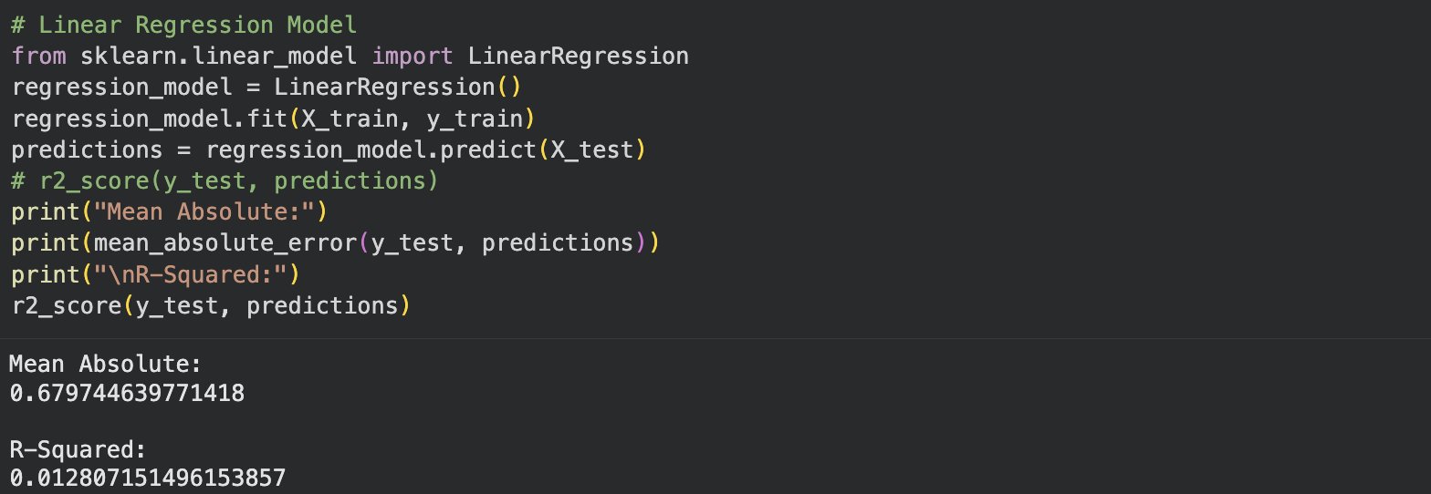The resulting mean absolute error and R^2 scores of the data space using linear regression. The mean absolute error score being \~0.68, and the R^2 score being \~0.01, both fairly bad scores showing little to no correlation.

Conclusions

Due to the similarity between star forming regions it is possible to conclude that Earth isn't too much of an anomaly, and all star forming regions have the possibility of producing one. Clustering algorithms were unable to find any believable groups essentially meaning that there aren't distinct groups or types.

Future Work

Something notable to mention is overfitting where the algorithm becomes too familiar with the dataset. By comparing WCO (Integrated CO admisssions, to S or the physical area of the cloud is in parsects you can adresss the question of "how many different life forming environments are there in the milky way?"

By using supervised regression we can put WCO as a function of surface density, physical area, physical size, mass, distance to the galactic midplace, galactocentric. This will answer how non-linear the relationship between CO and other molecular cloud features is and in turn answer how complex the relationship between organic molecules and other molecular cloud properties is. In simple, this answers "How complex can the building blocks of life be?"

1. Miville-Deschenes\, Marc-Antoine & Murray\, Norman & Lee\, Eve. (2016). Physical properties of molecular clouds for the entire Milky Way disk. The Astrophysical Journal. 834. 10.3847/1538-4357/834/1/57.

2. “Molecular Clouds - an Overview | Sciencedirect Topics.” Science Direct, www.sciencedirect.com/topics/earth-and-planetary-sciences/molecular-clouds. Accessed 6 Feb. 2026.

3. Maruyama\, Shigenori\, et al. “Nine requirements for the origin of Earth’s life: Not at the Hydrothermal Vent\, but in a nuclear geyser system.” Geoscience Frontiers, vol. 10, no. 4, July 2019, pp. 1337–1357, https://doi.org/10.1016/j.gsf.2018.09.011.

4. “Interstellar Medium and Molecular Clouds.” Interstellar Medium and Molecular Clouds | Center for Astrophysics | Harvard & Smithsonian, www.cfa.harvard.edu/research/topic/interstellar-medium-and-molecular-clouds. Accessed 5 Feb. 2026.

5. “Milky Way Molecular Clouds from CO Measurements - NASA Open Data Portal.” NASA\, NASA\, data.nasa.gov/dataset/milky-way-molecular-clouds-from-co-measurements.

6. Remick\, K. A.\, & Helmann\, J. D. (2023). The elements of life: A biocentric tour of the periodic table. Advances in microbial physiology, 82, 1–127. https://doi.org/10.1016/bs.ampbs.2022.11.001

I’m deeply grateful for my mentor PhD Tony Rodrigez for their guidance and encouragement throughout this project, as well as the knowledge he provided which served as a foundation for this study.