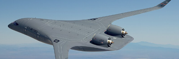
Blended Wing Aircraft, Financial Friend or Foe?
Grade 7
Presentation
No video provided
Hypothesis
Our hypothesis is that because of the more efficient shape, our 3d model of a blended wing aircraft will generate less drag, and therefore reduce the cost of gasoline or diesel. Meanwhile, the blended wing aircraft will also be more expensive to build and maintain because of the efficient and unique parts needed. It is also important to acknowledge the extra weight from the many passengers on board a commercial aircraft, because the engines would need more power, which also means that the plane would use more fuel.
Research
Bernoulli’s Principle:
- “Bernoulli's principle: Within a horizontal flow of fluid, points of higher fluid speed will have less pressure than points of slower fluid speed.” (Khan Academy, n.d.)
- “The key is the wing must deflect air downwards. This can be achieved using asymmetric or cambered airfoils, or by increasing the angle of attack.” (Ck-12, 2025)
What affects the cost of an airplane:
- “Aircraft structures must be light yet strong and stiff enough to resist the various forces acting on an airplane during flight. They must also be durable enough to withstand these forces over the airplane’s entire life span.” (How things fly, n.d.)
- “it appears that the structure of an airplane made by stick-and-wire-and-fabric or welded steel-fabric construction ranges from about three and one-half to four and one-half dollars per pound and for the whole airplane (light weight), including engine, propeller, and instruments, this figure ranges from four to five dollars per pound,” (n.d., 1936)
What affects the efficiency of an airplane:
- “aircraft weight, atmospheric conditions, runway environment, and the fundamental physical laws governing the forces acting on an aircraft.“ (Federal Aviation Administration, n.d.)
- “Long narrow wings, with the same wing area, generally allow for faster and more efficient flight than short stubby wings, because the wing tip area is reduced relative to the whole wing which in term reduces the formation of parasitic tip vortices.” (Krossblade Aerospace Systems, 2022)
- “These are small extensions at the tip of the wing that reduce the formation of parasitic tip vortices by creating a barrier for the high pressure air below the wing. This is preventing most of this high pressured air from leaking out to the top side of the wing - which would be an energy loss - thereby making the wing more energy efficient.” (Krossblade Aerospace Systems, 2022)
- “The primary factors most affected by performance are the takeoff and landing distance, rate of climb, ceiling, payload, range, speed, maneuverability, stability, and fuel economy.” (Federal Aviation Administration, n.d.)
- “The classically shaped regional and narrow-body-class BWBs offer only a marginal fuel-burn benefit relative to the equivalent conventional designs. The wide-body-class BWB offers up to 10.9% lower fuel-burn than the equivalent CTW.” (Reist & Zingg, n.d.)
Lift and Drag:
- “When thrust and drag are equal and opposite, the airplane is said to be in a state of equilibrium. That is to say, it will continue to move forward at the same uniform rate of speed. (Equilibrium refers to steady motion and not to a state of rest).” (MacDonald & Peppler, 2000, 21)
- “If the thrust is greater than drag the airplane will accelerate or gain speed. If drag is greater than the thrust, the airplane will decelerate or lose speed.” (MacDonald & Peppler, 2000, 21)
- “The equation says that lift is equal to the lift coefficient times the dynamic pressure times the wing area. Lift coefficient can be thought of as a measure of how efficiently the wing is transforming dynamic pressure into lift.” (Smith, 1985, 35)
- “Interference drag comes from the intersection of airstreams that creates eddy currents, turbulence, or restricts smooth airflow. For example, the intersection of the wing and the fuselage at the wing root has significant interference drag.” (Chapter 5 Aerodynamics of Flight, n.d.)
- “Form drag is the portion of parasite drag generated by the aircraft due to its shape and airflow around it. Examples include the engine cowlings, antennas, and the aerodynamic shape of other components. When the air has to separate to move around a moving aircraft and its components, it eventually rejoins after passing the body. How quickly and smoothly it rejoins is representative of the resistance that it creates, which requires additional force to overcome.” (Chapter 5 Aerodynamics of Flight, n.d.)
- “The lift and drag coefficients usually cap out at 2.” (Bayly, n.d.)
Pressure:
- “There are two ways to look at pressure: (1) the small scale action of individual air molecules or (2) the large scale action of a large number of molecules.” (Glenn Research Center, 2021)
Variables
|
Controlled |
Responding |
Manipulated |
|
|
|
Procedure
- Create an account with SimScale.
- Open a “New Project”.
- Title the project.
- On GrabCAD, find this NASA X-48B Blended Wing 3D model: https://grabcad.com/library/blended-wing-boeing-x-48-1.
- Download the 3D model and upload it onto the database in STEP format.
- Click on the geometry and click “Edit In CAD Mode”.
- Hover over the “Flow Volume” icon, and click “External”.
- Set the minimum and maximum dimensions based on the cord length (we used [in length 60m in the X direction, 90m in the Y direction, 90 m in the Z direction], [in the minimum directions -30m in the -X direction, -45 in the -Y direction, -30m in the -Z direction], [and in the maximum directions in the -X direction we used 30m, in the -Y direction we used 45m, and in the -Z direction we used 60m]).
- Click “Apply”.
- Go to “Delete”, select the geometry uploaded, click “Apply”, then click “Finish”.
- Click on the copy of the geometry you created, and then click “Create Simulation”.
- Select “Incompressible”.
- Set the “Turbulence model” to “k-omega SST”.
- Set the “Time dependency to “Steady-state”.
- Click the plus sign by “Materials”, therefore adding a new material to the simulation.
- Select “Air”, and set the “Assigned Volumes” to “Flow region”.
- Click on “Initial conditions”, and change the “Gauge pressure” to 0 Pa.
- Click on “Velocity”, and set everything to 0 meters per second.
- Click on “Turb. kinetic energy”, and set it to 0.00375 m2/s2.
- Click on “Specific dissipation rate”, and set it to 3.375 1/s.
- Next, add a Boundary condition, and select the “Boundary conditions” type as “Wall”.
- Set the Velocity to “Slip”.
- Select the four faces of the rectangle that are not in front or behind the plane, and then save it.
- Create another boundary condition.
- Make a pressure outlet, and set the Pressure type to “Fixed value”, and the “Gauge pressure” to 1915 Pa, then select the face that is behind the plane.
- Create another Boundary condition, and this time select “Velocity inlet”, then set the Velocity type to “Fixed value”, then set UZ to 55.56 m/s (two hundred Kilometers an hour), and then select the face that is in front of the plane.
- Save it.
- Select all the faces of the “Flow region”, right-click, and then click “Hide selection”.
- Draw a box around the plane, and then click the “Topological Entity Sets”.
- Then click “Create new set”.
- Create a new boundary condition, select “Wall”, set the Velocity to “No-Slip, set the “Turbulence wall” to “Wall function”, and then assign your “Topological Entity Set” that you created, and save.
- Go into “Advanced concepts”, select “Simulation control”, set the End time to 1000 seconds, the “Number of processors” to “Automatic”, the “Maximum runtime” to 20000 seconds, and then set the “Decompose algorithm” to “Scotch”, and save.
- Click on “Mesh” and set the Sizing to “Automatic”, Fineness to 5, turn on “Physics-based meshing” and “Hex element core”, turn off “Automatic extrusion meshing”, set the Number of processors to “Automatic, and the Maximum meshing runtime to 18000 seconds, then save.
- Click the plus beside “Simulation Runs”, and click “Run”.
Observations
Analysis
Conclusion
Application
Sources Of Error
Citations
References
(1936, February). Factors Affecting the Cost of Airplanes. Retrieved January 12, 2025, from https://pdodds.w3.uvm.edu/research/papers/others/1936/wright1936a.pdf
Bayly, D. (n.d.). [A interview with Donald Bayly (PhD in Mechanical Engineering)]. The Hanger Flight Museum, Calgary, Alberta, Canada.
Bernoulli's equation (article). (n.d.). Khan Academy. Retrieved November 30, 2024, from https://www.khanacademy.org/science/properties-of-matter-essentials/x56fba1647ecc4dbb:how-does-a-cricket-bowler-make-the-ball-swing/x56fba1647ecc4dbb:how-does-a-cricket-bowler-make-the-ball-swing-lesson/a/what-is-bernoullis-equation
Chapter 5 Aerodynamics of Flight. (n.d.). PHAK Chapter 5. Retrieved March 20, 2025, from https://www.faa.gov/sites/faa.gov/files/07_phak_ch5_0.pdf
Efficiency and Speed of Airplanes — Krossblade Aerospace Systems. (2022). Krossblade Aerospace Systems. Retrieved November 30, 2024, from https://www.krossblade.com/efficiency-and-speed-of-airplanes
Glenn Research Center. (2021, May 7). Dynamic Pressure. National Aeronautics and Space Administration. Retrieved March 15, 2025, from https://www.grc.nasa.gov/www/BGH/dynpress.html
MacDonald, S. A.F., & Peppler, I. L. (2000). From the Ground Up Millenium Edition (28th ed.). Aviation Publishers Co. Limited.
PHAK Chapter 11. (n.d.). Federal Aviation Administration. Retrieved November 30, 2024, from https://www.faa.gov/sites/faa.gov/files/13_phak_ch11.pdf
PHAK Chapter 11. (n.d.). Federal Aviation Administration. Retrieved January 12, 2025, from https://www.faa.gov/sites/faa.gov/files/13_phak_ch11.pdf
Reist, T. A., & Zingg, D. W. (n.d.). Aerodynamic Design of Blended Wing-Body and Lifting-Fuselage Aircraft. Retrieved March 20, 2025, from http://oddjob.utias.utoronto.ca/dwz/Miscellaneous/reistaviation2016.pdf
Smith, H. (1985). The Illustrated Guide To Aerodynamics (1st ed.). TAB BOOKS Inc.
12.5 Bernoulli's Law. (2025, March 1). Ck-12. Retrieved November 30, 2024, from https://flexbooks.ck12.org/cbook/ck-12-middle-school-physical-science-flexbook-2.0/section/12.5/primary/lesson/bernoullis-law-ms-ps/?referrer=search
University of Calgary Department of Microbiology Mentorship Program. (n.d.). Calgary, Alberta, Canada.
Weight and Strength | How Things Fly. (n.d.). for How Things Fly. Retrieved November 30, 2024, from https://howthingsfly.si.edu/structures-materials/weight-and-strength-0
Acknowledgement
We would like to thank Cayley Webber (Teacher), for setting up Science Fair at our school last year, Janet Summerscales (Teacher, Parent), David Bopp (Parent) and Susanna Santala (Collections Director at The Hangar Flight Museum, Parent), and the University of Calgary Mentorship Program, for their guidance in this project. On top of that, we thank Janelle Fortmuller (Teacher), for allowing us to work on our Science Fair project during Google Hour, and lastly, Donald Bayly (PhD in Mechanical Engineering, volunteer at The Hangar Flight Museum) for meeting with us and helping us understand certain equations and helping us with our research. We also thank SimScale, for sponsoring us so that we could use their simulation website for free, using an Academic Account (300 Core Hours, 1 year).