Minimizing time series forecasting error by considering a novel combination of factors to improve predictive accuracy
Grade 11
Presentation
Problem
A time series variable is a quantitative value that changes over time. For example, the average temperature in a city is a time series variable. Time series forecasting is the task of using statistical and/or machine learning models to predict the future values of a time series variable. This task has applications in almost every industry, ranging from business to healthcare (Tableau, n.d.).
Two popular neural network models for time series forecasting are the Recurrent Neural Network (RNN) and the Long-Short Term Memory (LSTM). A RNN is a series of cells which pass on time context in the form of a hidden state (Figure 1). It works similar to a deep neural network, with the exception that inputs are with respect to time and that the weights are the same for all layers (IBM, n.d.). RNNs are less widely used due to the vanishing and exploding gradient problems, making them quite difficult to train (Sharkawy, 2020).
The RNN struggles to capture long range relationships in time series data. A LSTM is a modified RNN that uses cells, made up of gates, to selectively learn and forget information from the data (IBM, n.d.). In this way, the LSTM can better retain information over long sequences, and make better predictions.
Previous studies have used machine learning models in combination with technical indicators tend to employ LSTMs or CNNs (Li & Bastos, 2020). Additionally, studies that use a combination of models tend to use each model for a different purpose, such as one model for feature extraction and another for prediction. Furthermore, different papers proposed different ways of integrating technical indicators into models. One paper trained a separate LSTM for each of 3 technical indicators (RSI, MACD, and SMA) (Sang & Pierro, 2019). However, we believe that including multiple technical indicators in the same model can improve model accuracy. Another paper normalized five technical indicators and then trained a BiLSTM with attention (Lee et al., 2022). The BiLSTM’s predictions were used in a simple stock trading strategy to decide whether to buy or sell a stock. This paper achieved a maximum accuracy of 68.83% for stock trend prediction. Due to the moderate accuracy achieved in this paper, we decided to use attention in our model as well. Lastly, another paper introduced a novel “Time Neural Network” which uses a kernel filter and a time attention mechanism to achieve low loss (Zhang et al, 2023). The kernel filter acts as a convolution and was used to better represent the input data, while the time attention mechanism used a separate neural network to generate attention weights. This paper tested the time neural network against other models and found that the time neural network worked best. As Zhang et al. (2023) discusses, a limitation of this study was to look at lagged relationships, which we improve in our model. Furthermore, we believe that attention weights should be generated within the model, such that the total back-propagation complexity should decrease.
Although most previous research combining machine learning models and technical indicators for time series forecasting focus on applications for stock price prediction, we believe that this method of forecasting can be generalized for all time series forecasting tasks. We believe this due to the promising results from previous studies, which suggest that a well developed model could learn complex relationships in time series data.
As such, this research aims to accomplish four main goals:
- Achieve a Mean Absolute Error (MAE) of less than 0.2σ on the testing data.
- Reduce training time on relatively large datasets.
- Create a model that does not require more than 5000 training examples to achieve the required predictive accuracy, which also uses technical indicators.
- Create a generalizable model (a model that does not use extra data, other than the original time series data, for prediction).
Method
Three datasets, collected from Kaggle, were used for training and testing the model. The first dataset was a Coca-Cola stock price dataset that contained stock prices from 1962-present (Rahman, 2023). The second dataset was a dataset of room temperatures collected from an IOT device (Madane, 2023). The third dataset was a dataset of daily confirmed COVID cases in Kerala, India from January 31st 2020 to May 22nd 2022 (Anandhu, 2022).
These three datasets were chosen to evaluate two main aspects of the model, its ability to predict a volatile or non-volatile time series variable and its ability to predict a cyclic time series variable, two common patterns that we expect a good model to be able to learn. Thus, the first dataset was used to test if the model could learn a relatively stable growth pattern, the second dataset was used to test if the model could learn cyclic patterns, and the third dataset was used to test if the model could learn a combination of both.
Furthermore, an electroencephalogram (EEG) dataset was collected. EEG data records electrical signals or waves in the brain, essentially measuring brain activity (Mayo Clinic, 2022). It is useful for medical diagnosis of diseases such as brain tumors and epilepsy. In this dataset, 100 subjects experienced epileptic seizure during recording (Andrzejak et al., 2001). Out of the 100 subjects, one subject's data was used to train and test models. This dataset could be used to identify patterns in EEG data of patients with epileptic seizures to help predict if and when future seizures could take place or can help with diagnosis.
Data collection procedures:
- Data was collected from the respective Kaggle datasets.
- Data was cleaned. Missing values and NaNs (not a number) will be replaced by the mean of the previous and next valid values.
- Technical indicators were calculated for the time series data. Technical indicators were calculated using the TA library in python.
The following technical indicators were chosen:
- Kaufman’s Adaptive Moving Average (KAMA): This technical indicator is used to deal with noise in time series data and can help identify the general trend (Padial, 2022).
- Bollinger band high and low: This technical indicator is used to identify the value range (high and low) of a time series with a specified number of standard deviations from the moving average (Hayes, 2023). This indicator was used to help the model to detect unusual movements.
- Aroon: This technical indicator is used to predict when the stock movement is likely to reverse (Padial, 2022). This indicator was included to teach the model to learn possible trend reversal signs.
- Moving Average Convergence Divergence (MACD): This indicator is the difference between two moving averages with different periods (Padial, 2022). It is used to identify possible signs of trends. This indicator was used to teach the model to follow trends.
- Triple Exponential Average (TRIX): This indicator calculates the change of a triple exponentially smoothed moving average (Chen, 2022). This indicator helps the model focus on important patterns and to predict the correct magnitude of increase or decrease.
The first 43 rows will be removed since the technical indicator calculations will cause these values to become undefined. Note: the number 43 was chosen, because the TRIX indicator is undefined until row 43. Then, the inputs were normalized by calculating the z-score for each of the 7 technical indicators. Furthermore, the inputs were batched into sequences of length 50, with 7 technical indicators for each training example. In a similar way, the testing dataset was created.
For the BEDCA inputs, the difference between each two consecutive z-scores was calculated and used as the input and testing data. This was done to ensure that the BEDCA captured the relationships better.
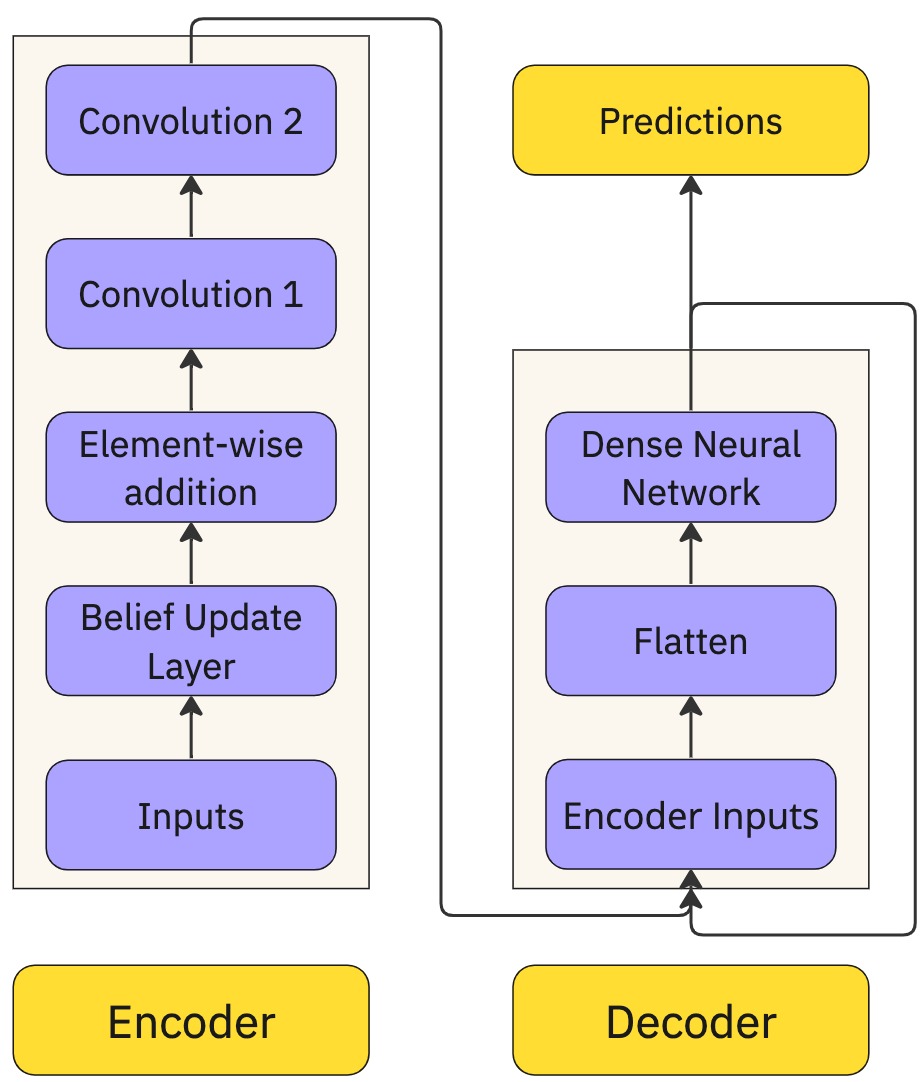
An overview of the model is shown in the figure above.
The forward propagation of the model works as follows: The input is split into training examples of shape (50, 7). This means that there are 50 time series values of 6 technical indicators and the actual time series data. For each training example, the next two values are the y values (outputs). This means that the aim of the model is to predict the next two values given a set of 50 preceding values.
Each technical indicator (including the actual time series data) in each training example, Xi, is input to a belief update layer. A belief update layer takes a matrix X of size 1 × 50 and calculates xT · x, resulting in a 50 × 50 matrix. This belief matrix captures lagged relationships in the input. Then, a convolution is performed with 8 filters, a kernel size of 4, and a stride size of 2 (no bias). This convolution acts as an attention mechanism, with each filter acting as a query to learn a separate relation in the belief matrix. Thus, no bias was used. These operations combine to form the belief update layer for a single technical indicator (including the actual time series data).
A belief update layer was applied to each of the 7 technical indicators separately. Element-wise addition was performed on the outputs for each of the technical indicators to obtain a tensor with shape (24, 24, 8).
On this, a convolution was performed with 16 filters, a kernel size of 3, and a stride size of 1. Subsequently, another convolution was performed on the output of the previous convolution. This convolution layer has 32 filters, a kernel size of 2, and a stride size of 2. Finally, max pooling was applied on the result, giving an Encoder representation of the input sequence. The above operations form the Encoder block.
The output of the Encoder was passed to the Decoder. The Decoder flattens its input and feeds it into a DNN (Dense Neural Network) with 1024, 256, 128, 32, 4, and 2 output units in its six layers. The relu, tanh, elu, and linear activation functions were used. The final two outputs of the DNN were the predicted outputs for the next two time steps (still normalized and differenced).
The loss function, which the model tries to minimize, is defined as:
![]()
This loss function ensures that the model is also trying to optimize its predictions for the long term, which is more desirable.
Analysis
From the results, it is evident that the BEDCA has a lower MAE for all three datasets analyzed. The MAE for the BEDCA is 25.9%, 58.7%, and 31.0% lower for each dataset respectively. These results also indicate that the BEDCA is able to learn low and high volatile data well, but struggles to learn cyclic data. Furthermore, it can be observed from the prediction images that the BEDCA’s predictions have a higher variance compared to the LSTM’s predictions. The BEDCA’s predictions are able to take into account more variation in the data, giving BEDCA the ability to learn and predict from more volatile data. This is most evident in the COVID cases data, where the LSTM was unable to predict significantly higher or lower values, while the BEDCA was able to predict with more success. Additionally, in all three of the BEDCA’s training loss graphs, it was seen that the loss was still decreasing. Thus, if trained for more epochs, the BEDCA would almost certainly have performed even better. This was not done due to computational resource limits.
Although the BEDCA was significantly more complex than the LSTM, it trained in a relatively short amount of time when compared to the LSTM. On all three datasets, the BEDCA took less than 3.5 times the amount of time taken for the LSTM to train, although the BEDCA was more than 35,000 times larger. The BEDCA also trains significantly faster than the Transformer. According to Anthony et al. (2023), τT=6PD, where τ![]() = FLOPs performed by the training hardware, T = amount of training time, P = number of parameters in the model, and D = the dataset size. Holding τ
= FLOPs performed by the training hardware, T = amount of training time, P = number of parameters in the model, and D = the dataset size. Holding τ![]() and D constant, we see that T∝P. Assuming a comparable transformer model contains 15-20 million parameters, the BEDCA trains 5 to 6.7 times faster.
and D constant, we see that T∝P. Assuming a comparable transformer model contains 15-20 million parameters, the BEDCA trains 5 to 6.7 times faster.
These observations pertain to the first three datasets. As for the EEG data, the BEDCA took 8 hours to train, while the N-BEATS took 36 minutes. Furthermore, from the results, it can be seen that the BEDCA performs significantly better than the N-BEATS model for the forecast horizon of 2. However, the BEDCA has slightly lower Symmetric Mean Absolute Percentage Error (SMAPE) than the N-BEATS but slightly higher Mean Squared Error (MSE) for the forecast horizon of 10. This indicates that the error for the BEDCA compounds quickly. However, this could also be due to the fact that the N-BEATS model is specifically trained for a certain input length, thus focusing more on prediction of this length. On the other hand, the BEDCA does not focus on a particular prediction length. Looking at the N-BEATS prediction versus the BEDCA prediction for the forecast horizon of 10, it is evident that N-BEATS is able to faster adapt to the downtrend, while the BEDCA struggles with this, being much more accurate in the first few predictions, and less accurate in the last few. From the N-BEATS decomposition, the last 5 prediction time steps have a significant decrease due to seasonality, which is larger than the increase due to trend. Thus, it can be further inferred that BEDCA struggles with seasonality, but is able to capture the trend accurately.
Conclusion
The results and analysis indicate that the BEDCA performs significantly better than the LSTM, and is a more practical choice than the Transformer. It also performs quite well when compared to the N-BEATS for short term forecasting, but it approximately equals N-BEATS for longer term forecasting.
Going back to the four goals laid out at the beginning of this paper, the MAE for the BEDCA were 6.41%, 22.07%, and 14.57% of the standard deviations of the respective datasets. From these, we can see that the BEDCA achieves the first goal (achieving a low MAE) for the first and third datasets. The BEDCA marginally missed this goal for the second dataset. This goal could have almost certainly been achieved if the BEDCA was trained for more time, since the loss was still decreasing. However, the second goal (reducing training time) was not achieved, as the BEDCA took longer to train than the LSTM on all three datasets. As for the third goal (using fewer than 5000 training examples), the BEDCA only used 1000 training examples for the first two datasets and 400 training examples for the last dataset. Since it was able to predict quite accurately using fewer than 5000 training examples, this goal was met. Lastly, the fourth goal (creating a generalizable model) was met, since the BEDCA is a generalizable model, as it was used for four different datasets. Furthermore, BEDCA was more generalizable than N-BEATS, since BEDCA could forecast for a variable number of time steps, but N-BEATS could only forecast for a specified number of time steps.
Through the observations made, two significant future considerations could be explored:
1. Decreasing training time:
Considering an efficient algorithm to backpropogate sparse weights could significantly reduce training time, since most of the BEDCA weights were close to 0. Furthermore, I could consolidate multiple operations into one larger, but simpler operation, so that the model performs even simpler operations, thus allowing it to improve faster.
2. Extending the EEG data:
The BEDCA could be trained on more patients to learn more possible relationships in patients who experience epileptic seizures. Then, this could be used to forecast if and when epileptic seizures occur by forecasting future values of EEG data of patients. Such a forecasting method could also be combined with other models, such as N-BEATS, to get the best of multiple models.
Citations
Andrzejak, R. G., Lehnertz, K., Mormann, F., Rieke, C., David, P., & Elger, C. E. (2001, November 20). Indications of nonlinear deterministic and finite-dimensional structures in time series of brain electrical activity: Dependence on recording region and brain state. Physical Review, 64(6). https://doi.org/10.1103/physreve.64.061907
Anthony, Q., Biderman, S., & Schoelkopf, H. (2023, August 18). Transformer Math 101. EleutherAI. https://blog.eleuther.ai/transformer-math/
Chen, J. (2022, September 18). Triple Exponential Average (TRIX): Overview, calculations. Investopedia. https://www.investopedia.com/terms/t/trix.asp
Coca Cola stock - live and updated. (2024, January 28). Kaggle. https://www.kaggle.com/datasets/kalilurrahman/coca-cola-stock-live-and-updated/
EEG (electroencephalogram) - Mayo Clinic. (2022, May 11). https://www.mayoclinic.org/tests-procedures/eeg/about/pac-20393875#:~:text=An%20electroencephalogram%20(EEG)%20is%20a,lines%20on%20an%20EEG%20recording.
Hayes, A. (2023, September 30). Bollinger Bands®: What They Are, and What They Tell Investors. Investopedia. https://www.investopedia.com/terms/b/bollingerbands.asp
IBM. (n.d.). What are recurrent neural networks? https://www.ibm.com/topics/recurrent-neural-networks
Latest COVID-19 confirmed cases Kerala. (2022, May 22). Kaggle. https://www.kaggle.com/datasets/anandhuh/covid19-confirmed-cases-kerala
Lee, M. C., Chang, J. W., Yeh, S. C. et al. (2022, January 28). Applying attention-based BiLSTM and technical indicators in the design and performance analysis of stock trading strategies. Neural Comput & Applic 34, 13267–13279. https://doi.org/10.1007/s00521-021-06828-4
Li, A. W., Bastos, G. S. (2020, October 12). Stock Market Forecasting Using Deep Learning and Technical Analysis: A Systematic Review. IEEE, 8. https://doi.org/10.1109/ACCESS.2020.3030226
Oreshkin, B. N., Carpov, D., Chapados, N., & Bengio, Y. (2019, May 24). N-BEATS: Neural basis expansion analysis for interpretable time series forecasting. arXiv.org. https://arxiv.org/abs/1905.10437
Padial, D. L. (2022, August 23). Technical Analysis Library in Python Documentation. Technical Analysis Library in Python. https://technical-analysis-library-in-python.readthedocs.io/_/downloads/en/latest/pdf/
Sang, C., & Pierro, M. D. (2018, November 14). Improving trading technical analysis with TensorFlow Long Short-Term Memory (LSTM) Neural Network. The Journal of Finance and Data Science, 5(1), 1–11. https://doi.org/10.1016/j.jfds.2018.10.003
Sharkawy, A. N. (2020, August 20). Principle of Neural Network and Its Main Types: Review. Journal of Advances in Applied & Computational Mathematics, 7. https://doi.org/10.15377/2409-5761.2020.07.2
Tableau. (n.d.). Time Series Forecasting: Definition, Applications, and Examples. https://www.tableau.com/learn/articles/time-series-forecasting#::text=It%20has%20tons%20of%20p
Time series room temperature data. (2022, November 21). Kaggle. https://www.kaggle.com/datasets/vitthalmadane/ts-temp-1?select=MLTempDataset1.csv
View of Principle of Neural Network and its main types: Review — Journal of Advances in Applied & Computational Mathematics. (n.d.). https://avantipublisher.com/index.php/jaacm/article/view/851/502
Zhang, L., Wang, R., Li, Z., Li, J., Ge, Y., Wa, S., Huang, S., & Lv, C. (2023, September 13). Time-Series Neural Network: A High-Accuracy Time-Series forecasting method based on kernel filter and time attention. Information, 14(9), 500. https://doi.org/10.3390/info14090500
Acknowledgement
I sincerely thank Daniel Plymire for his continued support and my parents for their encouragement throughout the project.