
A Machine Learning Approach for Predicting Length of Stay at the Emergency Department
Grade 10
Presentation
Problem
In urban Alberta hospitals, the average number of hours in which patients stay in the Emergency Department (ED) is around 6 hours (Patient Emergency Department Total Length of Stay (LOS) | HQCA Focus, 2024). The length of stay is dependent on a variety of variables, including the severity of the patient’s condition and the crowdedness of the department. For some people, they may only stay in the ED for a few minutes, while some others may stay for up to 30 days. The current unpredictability of patient stay length creates the possibility of poor resource management, unstable expectations for patients, and disruptive patient flow in the department. The ability to forecast how long a patient will stay in the emergency department aids in resource allocation, capacity planning, and patient flow management, leading to both higher quality of care and more effective cost control. With the progressing advancement of Artificial Intelligence (AI), there is great potential to utilize this technology to predict the length in which a patient will stay in the ED. A common AI approach is a machine learning algorithm known as Random Forest, which combines multiple decision trees to make predictions. It aggregates the results of individual decision trees to improve accuracy and reduce overfitting, making it effective for tasks such as classification and regression (IBM, 2023). This project will utilize Random Forest to classify and predict patients’ stay times using basic patient characteristics and hospital information.
Method
Objectives
The primary objectives of this study were to:
- Predict whether a patient stays in the ED for more or less than:
- (a) 4 hours (government’s target stay time for patients who do not need admission into hospital)
- (b) 8 hours (government’s goal for patients who need admission into hospital)
- (c) 6 hours (average of the two goals)
- Predict the stay time to the minute.
The secondary objectives of this study were to:
- Determine the impact of using different time breaks for a two-category model.
- Determine the impact of using a different number of categories on a model.
- Determine the impact changing the number of trees (ntree) and number of variables considered at each split (mtry) have on the results.
- Determine the importance of variables and their impact on the prediction.
- Predict whether the patient is admitted into hospital, discharged, or other (left before being seen, etc.).
Dataset
Variables
The main dependent variable is the patient length of stay in minutes, which was measured from seeing the triage nurse until leaving the emergency department.
Random Forest
Random Forest is a machine learning algorithm that aggregates multiple decision trees, made through training them on subsets of data, to create a final prediction with the combination of all trees (IBM, 2023). Random Forest is capable of producing two distinct types of models: classification, which classifies data points into categories, and regression models, which predicts the exact value of a data point.
The number of decision trees created (ntree value) and the number of variables tried at each tree’s split (mtry value) are generally set to different values based on the type of model (Random Forests · AFIT Data Science Lab R Programming Guide, n.d.). This study utilized the package RandomForest in R version 4.3.2; for this package, the default for a classification model was that ntree = 500 and mtry = sqrt(p), with p being the number of variables. On the other hand, the default for a regression model was ntree = 500, and mtry = p/3 (p being the number of variables). Both the ntree and mtry values have an impact on the models’ accuracy.
Random Forest is capable of creating variable importance plots on its models, which reveal the relative importance of each variable to the prediction of the model (How Is Variable Importance Calculated for a Random Forest?, 2018). To find the impact of each variable on the models, partial dependence plots (PDP) were created which display how much the model may depend on each variable (Molnar, n.d.). PDPs may be 1-variable (only showing the dependency of one variable on the target variable) or 2-variable (showing the interconnected dependencies of two variables and the target variable).
Procedure
To resolve the first primary objective, 3 binary (2-category) classification models with their time breaks at 4, 6, and 8 hours were made, each with a mtry value of 2 and a ntree value of 500. Although those were the emphasized models according to the primary objectives, more models with different time breaks (two categories, time break from 1 hour - 12 hours), number of categories (from 1 - 10), ntree values (from 100 to 1000, increasing in intervals of 100, with mtry = 3) and mtry values (from 1 to 7, with ntree = 500) were created to resolve the first four secondary objectives. Another classification model was created to predict which category of disposition group (admitted to hospital, discharged from hospital, or other) to determine the results of the sixth secondary objective.
One regression model was additionally made for the second primary objective, where, for the fifth secondary objective, variable importance plots were created, as well as both 1-variable and 2-variable PDPs.
Research
Classification Model
The first type of Random Forest are classification models, where the algorithm assigned data points into a defined category. The performance of these models can be evaluated using the confusion matrix.
Figure 1. Confusion matrix of a two-category classification model.
In the confusion matrix, the predicted and actual values are evaluated, with true positive (TP) being the number of correctly predicted values of the first category and true negative (TN) being the values correctly predicted of the second category (Basic Evaluation Measures from the Confusion Matrix, 2015). False positive (FP) then refers to the number of values incorrectly predicted to be in the first category while, in actuality, being in the second; conversely, false negative (FN) is the number of values predicted to be in the second category when it is in the first. Because TP, TN, FP, and FN value is calculated for each category in a classification model, the number of columns and rows of the confusion matrix increases with the number of categories.
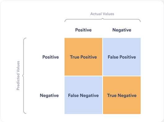
Using the confusion matrix, 4 different measurements can be calculated to evaluate the model’s performance (Basic Evaluation Measures from the Confusion Matrix, 2015). Positive predictive value refers to the total number of true positives in all of the positive predictions, which is calculated by TP / (TP + FP). Negative predictive value is the total number of true negatives in all of the negative predictions, calculated using the formula TN / (TN + FN). Sensitivity is calculated using the formula TP / (TP + FN). A high sensitity is an indicator that there are few false negative results, thus fewer cases of long stay are missed. It also means that it has less false negatives. Specificity uses the formula TN / (TN + FP). A high specificity indicates that the model is effective at correctly identifying instances of the negative class. It also means that the number of false positives is lower.
The accuracy of the model can then be calculated with the equation accuracy = (TP + TN)/(TP + FP + TN + FN). Conversely, the out-of-bag (OOB) error rate is found by separating the dataset into two sets, where the “out of bag” set is used to test the accuracy of the model as trained on the “bagged” set, to find the overall error rate (Out-of-Bag Error | Dremio, n.d.). The error rate of a specific category is shown at the end of the confusion matrix under “class.error”, where 0 = all correct predictions and 1 = all incorrect predictions.
Regression Model
Random Forest is also capable of creating regression models, where data is predicted by the algorithm to the exact value; in this study, the regression model would be predicting for the exact minute (Sruthi, 2021).
The model can be evaluated via the % variability explained, which is the amount of variability in the data that can be “explained” by the model (Wickramasinghe, n.d.). The residual is the difference between the model’s predicted value and its actual value, where, for each datapoint, there is a different residual (Taylor, 2019). The mean absolute error is the mean of the absolute value of the residuals, where the closer the mean absolute error is to zero, the better the model performs (Chugh, 2020).
Data
Dataset
Figure 2. Histogram of the distribution of length of stay, in minutes, for all data under the 90th percentile.
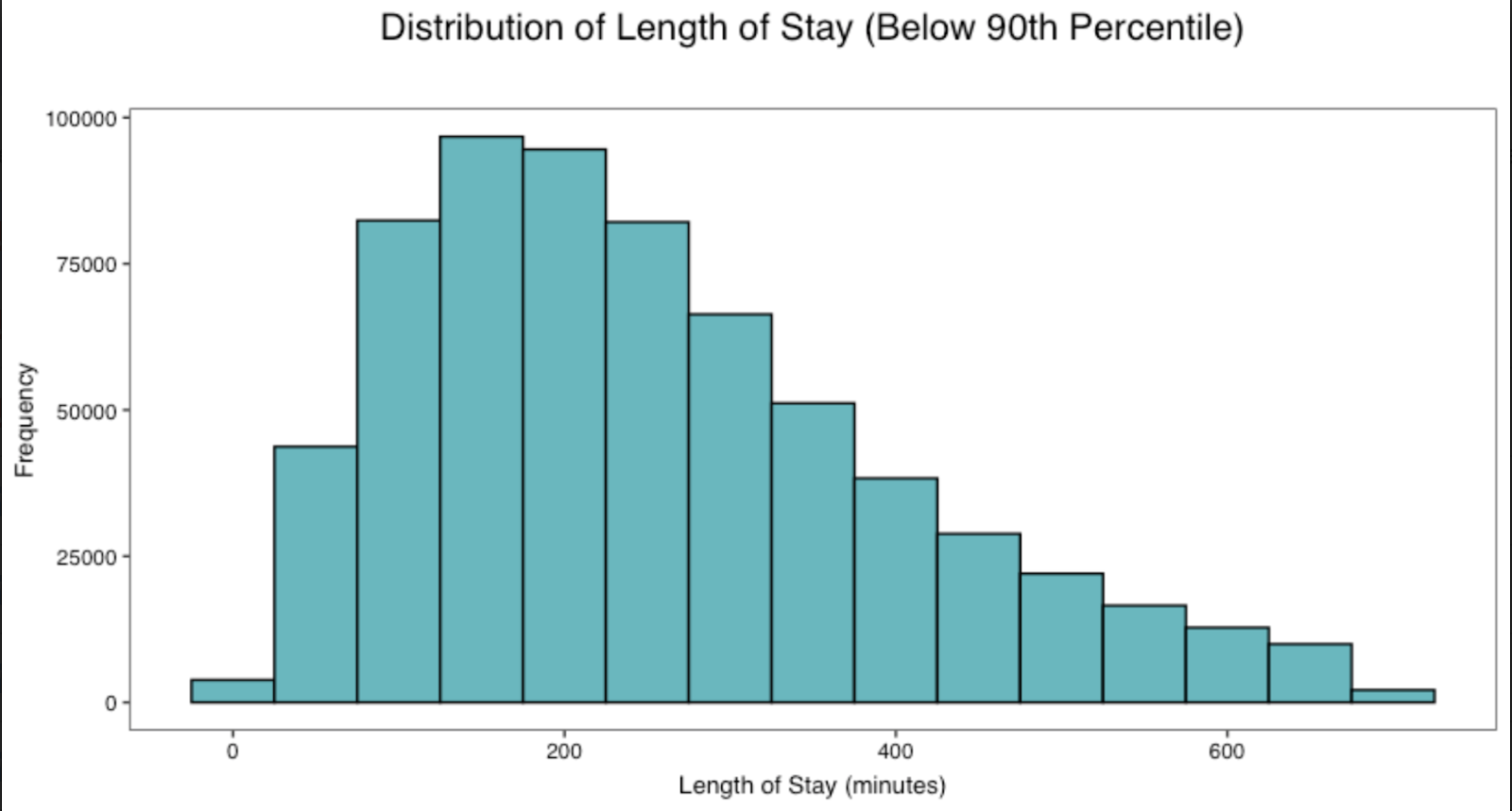
In this dataset, it was most common for patients to have a length of stay of roughly 150 minutes. On the other hand, it was least common for patients to have a length of stay of 700 minutes. However, it must be considered that, despite it being the least common, the y-axis of the graph is very extensive and there are still a substantial number of patients (25,000 or more) who have a 700 minute stay time.
Baseline Characteristics
Due to the length of the table, the baseline characteristics table has been externally linked as https://docs.google.com/document/d/1UsV3_H6ceoV2blitNScvAT3SbHeTClfWnYhoHXngCkU/edit?usp=sharing.
There is not a notable difference in the sex of the patients who come to the ED: both sexes make up roughly 50% of the data, both for the over and under 4 hours stay time categories. This indicates that there is not a significant difference in the possibility of either sexes going into the ED for any length of stay. There is a considerable difference of ED stay length for patients with different ages. For individuals in age group 1 (ages 1 - 5), 74.2% of age group 1 patients stay for less than 4 hours. On the other hand, out of those in age group 19 (ages 85 - 90), 83.2% of age group 19 patients stay for longer than 4 hours. This may suggest that, as people age, they develop more complicated medical histories or conditions that prolong their stay. Additionally, for the stay time for patients who had or had not had a previous hospitalization within the past 3 years, patients who had not had a previous hospitalization make up 70.2% of those who stay for less than 4 hours, and 56.9% of patients who stay for longer than 4 hours, accumulating to 63.3% of the total dataset.
Of all the ICD 10 categories, the highest number of patients were in categories 18 (unclassified symptoms and abnormal clinical/laboratory findings) and 19 (injury and poisoning). The lowest number of patients in the ICD 10 categories were of 16 (conditions from the perinatal period) and 17 (congenital malformations/deformations or chromosomal abnormalities).
The majority of patients in the ED have triage code (CTAS score) of 2 and 3, making up 26.4% and 48.6% of the dataset respectively, and most individuals who stay in the ED for levels 1, 2, and 3 stay for longer than 4 hours, while more patients in levels 4 and 5 stay for less than 4 hours. This suggests that the more severe the condition, the longer a patient stays, likely because the treatment is more complex and time-consuming. Moreover, many hospitals have a “fast track” to rapidly run patients with lower CTAS levels through the hospital, which likely contributes to most patients with lower triage levels having shorter stay times.
The institutional ID shows that, of all the 16 encoded hospitals, hospital 1 has the most patients having a stay time of less than 4 hours while being the hospital with the tenth most patients having a stay time over 4 hours. This suggests that hospital 1 either has efficient patient control or most patients going to hospital 1 have conditions that require less time to treat. Contrastingly, hospital 7, which had the most patients of any hospital, had the most patients over 4 hours and the second most number of patients of all patients with a stay time of less than 4 hours. In consideration of the number of patients coming from this hospital, the institution is likely urban, and may have moderate management and resource control, or most of the patients in the urban area going to the hospital generally have conditions that take longer to treat, or some combination of both.
For the baseline characteristics table, the 173 different types of patient district codes were collapsed into the categories “urban” and “rural”. Most patients of this dataset live in urban areas (95.2% of the dataset), and 46.5% come from large urban hospitals. With institutional peer groups, it is of note that more patients in large urban hospitals (the number of patients make up for 50% of the dataset) stay for more than 4 hours than for less. This suggests that urban patients may go to the ED for diseases that are more lengthy to treat, or that urban hospitals may have worse resource allocation and management suitable for its large number of patients. However, for large urban ambulatory and rural/suburban hospitals, there is a greater number of patients who have a stay time of less than 4 hours than for more, which indicates that, with smaller hospitals, the resource management may be more efficient or patients have conditions that take less time to treat.
Classification Model Results
Two-Category, 4 Hours Timebreak Model
Table 2. Confusion matrix for the two-category 4-hour timebreak classification model.

The accuracy of the model with 4 hours as the time break is 70.2% and, consequently, the OOB error rate is 29.8%. Comparatively, the model’s negative predictive value is 10.8% higher than the positive predictive value, indicating that out of all the negative class predictions made by the model, more were correct compared to the positive class predictions. The sensitivity and specificity have similar values, so the model has consistent performance for identifying both categories.
Two-Category, 6 Hours Timebreak Model
Table 3. Confusion matrix for the two-category 6-hour timebreak classification model.

Accuracy for the model with 6 hours as the time break is 75.9%, with a 24.6% OOB error rate. The PPV and sensitivity both indicate that this model is performing better with predicting the people with stay times of less than 6 hours.
Two-Category, 8 Hours Timebreak Model
Table 4. Confusion matrix for the two-category 8-hour timebreak classification model.

The accuracy of this model is 83.0%, demonstrating higher overall performance compared to the previous models. There is a considerable difference between the model’s ability to correctly predict the positive class and the negative class. As indicated by the PPV and sensitivity, it is significantly better at identifying patients with a stay time of less than 8 hours.
Classification Model Trends
Figure 3. Accuracy across two-category classification models with different numbers of trees tested.
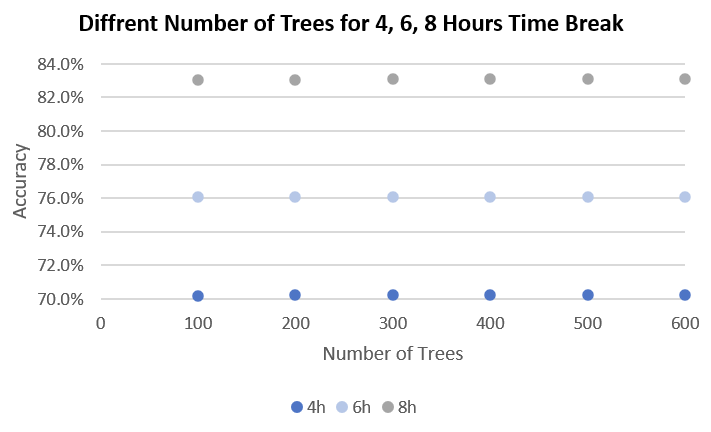
Figure 4. Accuracy across two-category classification models with different numbers of variables considered at each split.
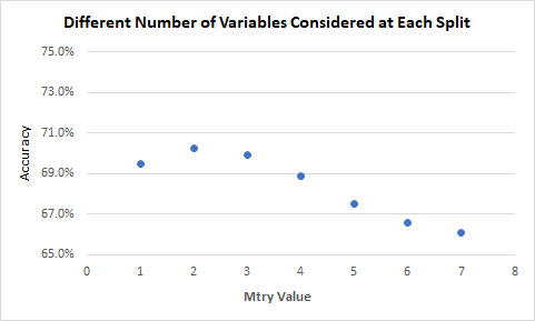
Although the results were mostly minimal, it can be seen that there is some impact that both mtry and ntree have on the accuracy of the model. Ntree had consistent accuracies across all values, while the mtry values were generally better at 2, although only by ~1%. These results somewhat align with the default values for ntree and mtry. However, due to the model only utilizing 8 variables and the formula for mtry being sqrt(p) (p being the number of variables, rounded down), different mtry values may have much higher impact on the accuracy with a larger number of variables.
Another trend was found between the classifications models: as the timebreak reaches an extreme (either long or short), the accuracy increases.
Figure 5. Accuracy across two-category classification models with 2, 4, 6, 8, 10, and 12 hour time breaks.
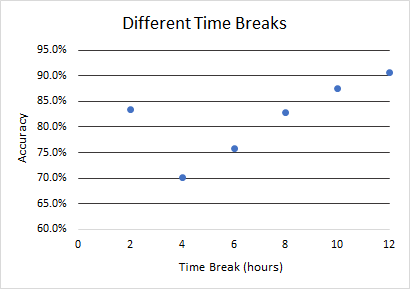
As the time break reached the median of the dataset (4 hours), it reached a depression: the accuracy dipped from the 2-hour timebreak model (nearly 85%) to 70%. After the 4 hour time break, the accuracy increases as the time break increases, with the highest accuracy being at the longest extreme end, being the models with a 12 hour timebreak. This is likely because, as the timebreak becomes more extreme, there is a high difference in the number of data points in the two categories, so the model classifies most of the data points in the category with more people. Since one category may have significantly more people than the other one, classifying most people into the larger category is more likely to be correct, thus increasing the accuracy. As seen in the confusion matrices for the models with 6 and 8 hours as the time break, the model becomes better at identifying the patients who stay less than the time break. For these two models, there are more people in the category of a short stay, meaning that most people are classified into that category, the predictions are more likely to be correct, thus increasing the overall accuracy.
Multiple models with a different number of categories were also considered, with the results summarized in the following graph:
Figure 6. Accuracy across classification models with 2, 4, 6, 8, and 10 categories.
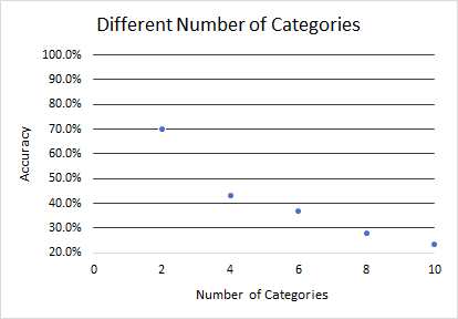
Across this graph, the general trend is observable: as the number of categories increases, the accuracy decreases, going from about 70% for a 2-category model to nearly 20% for a 10-category model. This is likely due to the large range of factors that contribute to the length of stay’s unpredictability, making it difficult for the model to classify accurately as the number of categories increase and the increment of each category decreases.
Characteristics of Misclassified Patients for 2-Category Classification Models
Due to the length of the table, the table has been externally linked at https://docs.google.com/document/d/1_fsHg4oqdEKuaCGWBZhMiYyLrjiU6LYVZZGQXtEtbaE/edit?usp=sharing.
Although most of the variables showed an increase in accuracy in the 6-hour timebreak model, the age group in table 5 show an interesting trend: for age groups 13 - 19 (ages 61 - 95), the accuracy decreases from the 4-hour timebreak model to the 6-hour timebreak model. According to the 1-variable partial dependence plot with age group, the length of stay for groups 13 - 19 are all, on average, longer than 6 hours. Generally, mid-younger age groups hold a greater number of people, and the youngest patients have generally shorter stay times than patients who are in older age groups. Mid-older patients, however, are concentrated around the 6 hour mark, with only the highest of age groups having a more obviously long stay time. Due to this, the 4-hour timebreak classification model would likely categorize most of the older patients into the above 4 hours category as most of them do stay for longer than 4 hours. However, there is less certainty with the 6 hour-timebreak model as the mid-older patients are highly concentrated around the 6 hour stay time mark. Thus, the model is more likely to classify them into the incorrect category. This is potentially why there is a slight decrease in the correct prediction rate when the age group is increased.
Similarly, for patients who have been previously hospitalized in the past three years, the incorrect predictions also increase when the time break increases. This may be as patients who have been previously hospitalized are more likely to have more severe and sporadic conditions. The 4-hour timebreak model is likely to classify most of them as staying longer than 4 hours, but the 6 hour-timebreak model has to predict the data with previously hospitalized patients who stay for just around 6 hours, thus making it more difficult to predict.
For triage code, levels 1 and 2 show the number of incorrect predictions as somewhat consistent but with a slight increase. This may be due to the unpredictability of the patients who fall under this category, as the stay time is more likely to vary for severe conditions. For levels 3 to 5, the conditions are not as severe and the time needed to treat them decreases, which is why patients are more likely to fall under the shorter than 6 hours category for the 6 hour-timebreak model, thus increasing the accuracy for these 3 triage code levels.
The percentages for sex, ICD categories and patient postal district displayed a nominal change from category to category, indicating that they have minimal impact on the accuracy of the predictions.
Disposition Group Prediction Model
This model had a confusion matrix as follows:
Table 6. Confusion matrix for the classification model predicting the disposition of a patient in the ED.

The accuracy of the model is 71.4%, with an OOB error rate of 28.6%. The model has shown higher performance at identifying the people who were discharged home. One reason may be that people who were not admitted into the hospital generally have less severe conditions, which may potentially be more predictable than people who were admitted into the hospital. Another possible explanation may be that there are more people who were discharged home compared to the other two categories. Since there are more people in the discharged category, the predictions made by the model are more likely to be correct, thus increasing the overall accuracy.
Regression Model
The regression model that was made displayed a 20.1% variability explained, with the minimum absolute residual being 0.001 minutes, the maximum absolute residual being 14525.4 minutes, and the mean absolute residual being 205.5 minutes.
Variable Importance
A variable importance plot was created on the regression model to demonstrate which variables contributed the most to the model:
Figure 7. Variable importance plot for the regression model.
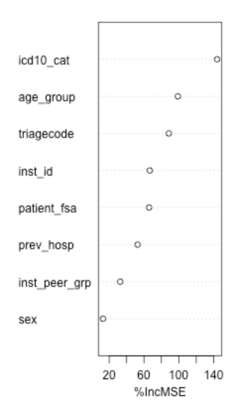
As shown by the plot, the most important variable was the ICD 10 category; the type of disease or injury thus has some impact on the length of stay of a patient. The age group suggests that a patient’s age is correlated with their ED stay time, as well as the severity of their condition as reflected in the triagecode. The institutional ID having some importance suggests that some hospitals may have conditions that cause longer or shorter stays than others (such as number of employees, location, etc.). The patient district code, in which their housing area could be correlated with their financial situation, shows to have moderate relation with the length of stay, suggesting that the economic status of a patient may impact the stay time. The previous hospitalization status has less of an impact on the model, suggesting that it does not contribute too much to a patient’s length of stay. The type of hospital has minimal importance to the model, this indicates that hospitals may generally provide similar services without regard to the type of hospital. Lastly, sex assigned at birth is the least important to the model, which suggests that there is likely no bias for patients based on their sex.
1-Variable Partial Dependance Plots
For the three most important variables, partial dependance plots (PDP) were created to show how the model predictions depends on each variable, such as for the ICD 10 category:
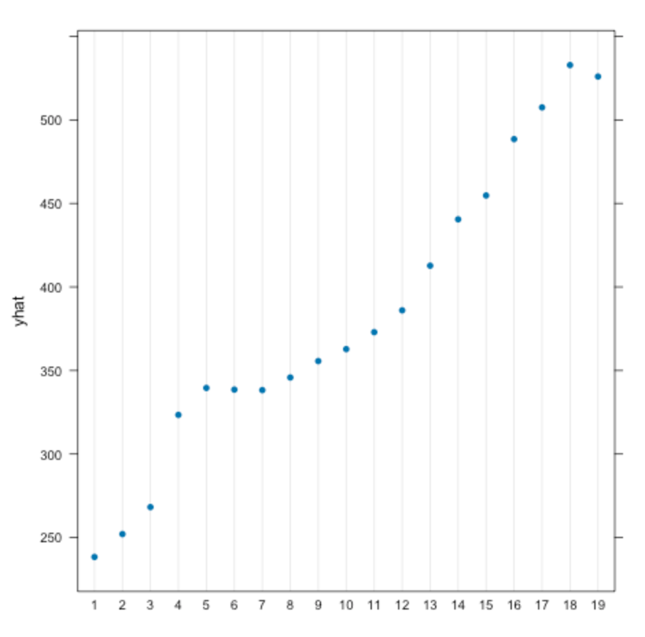
Figure 8. Partial dependance plot for the ICD 10 category.
The plot indicates that, of every ICD 10 category, the ones that have the longest length of stay, averaging more than 10 hours of stay time in the ED, are mental and behavioral disorders under category 5. However, categories 2 (neoplasms), 3 (diseases of the blood), and 4 (endocrine/nutritional/metabolic diseases) also constitute considerable ED stay lengths of ~520 minutes (8.7 hours). This may be because these are diseases or disorders that are difficult and lengthy to treat, or that it may require more observation and consideration for the treatment of. Conversely, the categories that lead to the shortest stay times are categories 7 (diseases of the eye) and 8 (diseases of the ear). This may be due to these diseases being those that require a shorter treatment, resulting in a shorter ED stay length.
Figure 9. Partial dependance plot for the age group.
The PDP for age group suggests that, as the patient’s age increases, their corresponding ED length of stay increases as well. It is of note that there is a large jump of ~90 minutes between age groups 3 (ages 10 - 15) and 4 (16 - 20). With 18 years old as the legal age, this difference may indicate a difference in wait time between regular hospitals and childrens’ hospitals. Another possibility is that, in general, children may just be more prioritized than adults in the emergency department.
Figure 10. Partial dependance plot for the triage code (CTAS score).
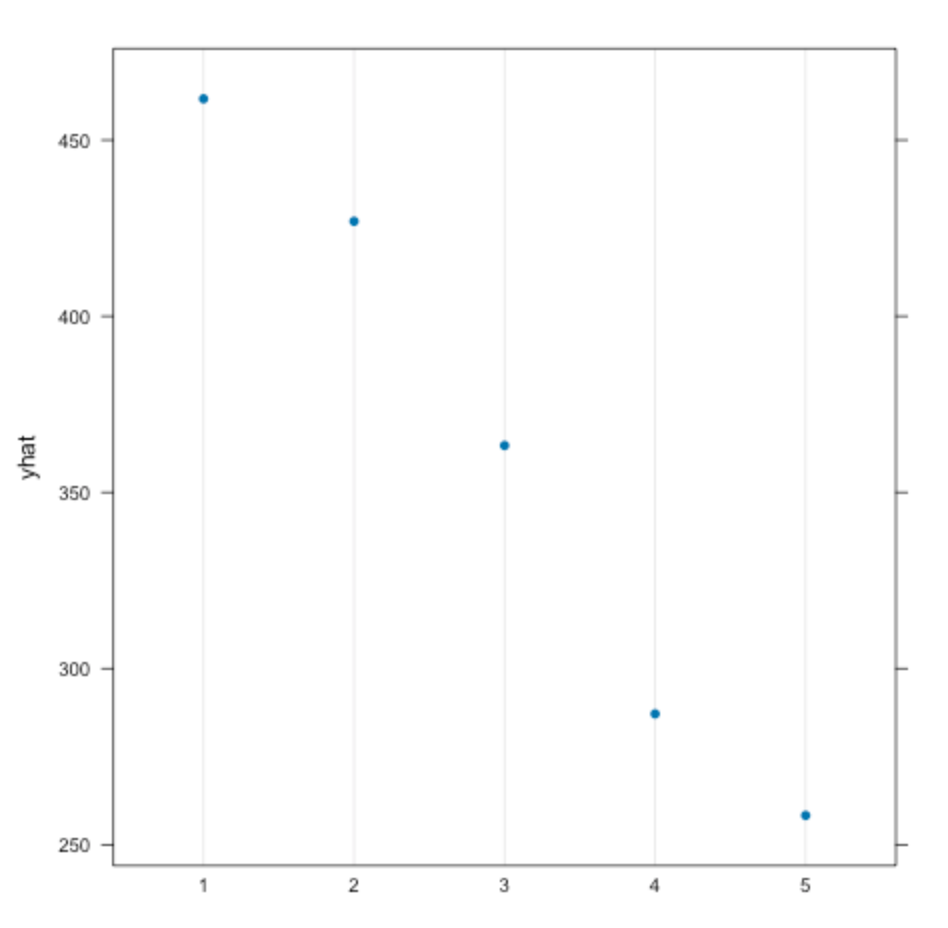
For the PDP for triage code (CTAS score), the indication was that patients with the most severe conditions have nearly double the length of stay as patients with the least severe conditions. This may be due to patients having more severe conditions requiring more complex and lengthy treatments as most high-urgency situations require immediate and lengthy action before it is possible for a patient to be transferred to another department. Contrarily, patients with the lowest scores and least severe conditions have the shortest ED stay time. This may be due in part to those patients requiring only small and fast treatments, and thus they may leave the emergency department faster. Another consideration is that this may be due to many hospitals having a “fast track” for patients with lower CTAS scores to manage them through the hospital’s system faster.
2-Variable Partial Dependence Plots
Figure 11. 2-Variable partial dependance plot for ICD 10 category and triage code, correlated with the predicted length of stay in minutes.
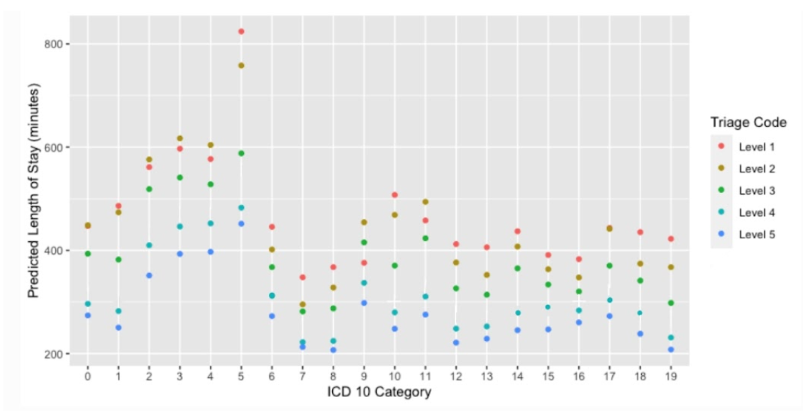
The PDP of ICD-10 categories and triage code levels show mostly sporadic points due to the ICD-10 categories being strictly classified and not progressive. The general trend shows that higher CTAS levels result in longer stay times, regardless of the ICD-10 category. However, the PDP shows an interestingly large spike in length of stay at category 5 (mental and behavioral disorders), of which the stay time increases as the severity increases. In consideration of the 1-variable PDP of ICD-10 category, where category 5 was the most lengthy condition to treat, this PDP indicates that the more severe the mental or behavioral disorder, the longer it will take to treat, especially for the most severe of cases. For other conditions, such as the ones for categories 6 (diseases of the nervous system), 7 (diseases of the eye), 8 (diseases of the ear), and 16 (conditions originating in the perinatal period), the difference in time between difference triage levels is small, suggesting that, regardless of severity, these are all conditions that take similar amounts of time to treat. Moreover, for categories 2 (neoplasms), 3 (diseases of the blood), 4 (endocrine, nutritional, and metabolic diseases), 9 (diseases of the circulatory system), 11 (diseases of the digestive system), and 17 (diseases of the skin), the predicted stay time is longer for triage level 2 more than 1. One possibility is that there are external factors, such as more patients having those conditions triaged as CTAS score 2 go to a busier hospital, or having other complications, which prolong their stay time longer than patients with those conditions and triage level 1.
Figure 12. 2-Variable partial dependance plot for triage code and previous hospitalization status, correlated with the predicted length of stay in minutes.
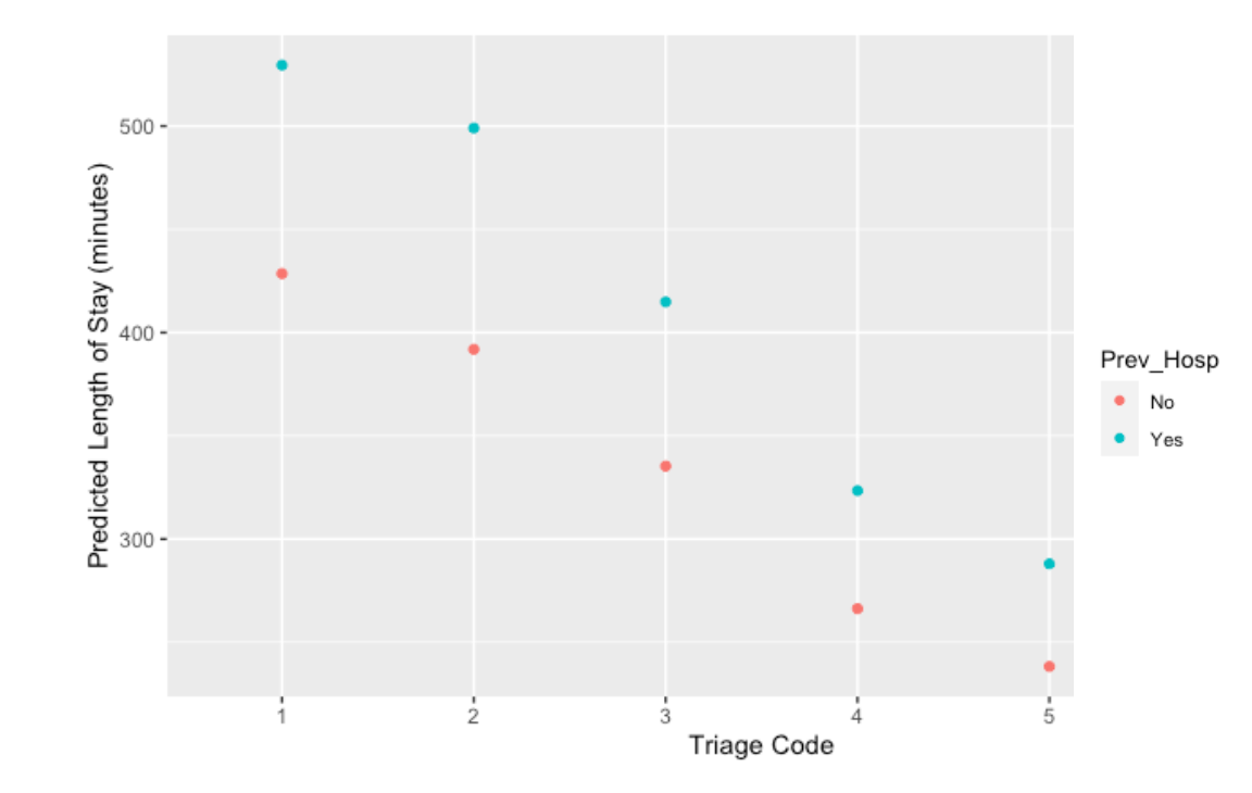
For this PDP of triage code and previous hospitalization status, there is an observable trend of the increase of triage levels (thus decrease of severity) being correlated with the decrease of stay time. However, it is noticeable that, for every triage code level, patients with a history of previous hospitalization stay, on average, just under 100 minutes longer than patients without. This suggests that, for all severities, there is a correlation between a patient’s previous hospitalization status and their wait time. The decrease of difference in predicted wait time between previously and not previously hospitalized patients with the increase of triage levels suggests that, in more severe cases, the previous hospitalization yields more impact on the stay length, while in less severe cases the previous hospitalization has less impact. However, it is of consideration that the majority of patients in the data are in CTAS score 2; the large distribution of data may be contributing to the difference in stay time between those who have and have not been previously hospitalized in this level.
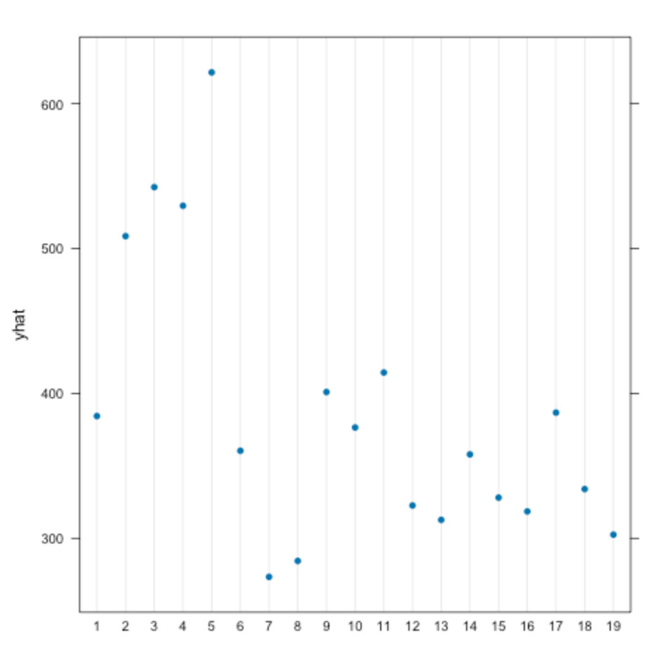
Figure 13. 2-Variable partial dependance plot for age group and triage code, correlated with the predicted length of stay in minutes.
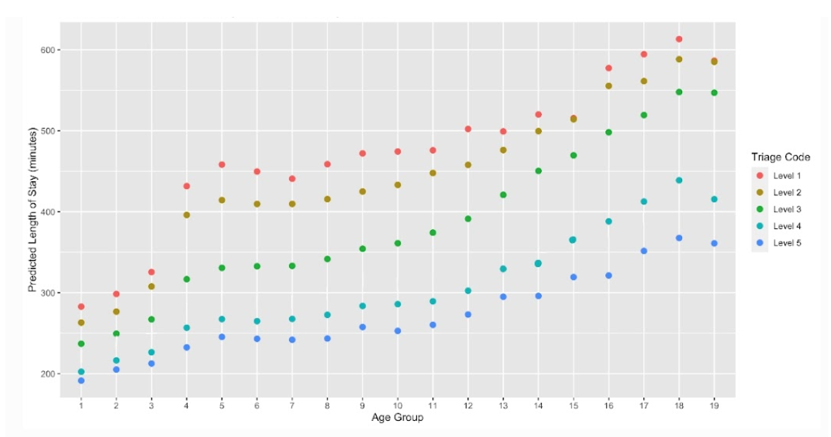
While the PDP of age group and triage codes shows a general trend of stay time increasing as the age group increases across all triage levels, there is a noticeable gap between the times of CTAS level 1 for age groups 3 (ages 11 - 15) and 4 (ages 16 - 20), with the latter having a roughly 100 minutes longer stay time. As these different groups outline the break between youth and adults, these results may be highlighting the different treatment between children and adults. It could be that children's hospitals have more effective management, resource allocation, and are overall more efficient than regular hospitals and are more prepared and prompt to remedy severe conditions; it could also be that regular hospitals may give children some priority ahead of adults, which is why there is such a great gap between the two stay times. The sporadicness of triage level 1 suggests that there are a variety of different factors and conditions that are correlated with the most severe conditions, causing the length of stay to be the most spread out. On the other hand, triage level 3, 4, and 5 are more linear and stable, indicating that for lower severities, the length of stay is more predictably longer as a patient grows older.
Figure 14. 2-Variable partial dependance plot for age group and sex, correlated with the predicted length of stay in minutes.
The PDP of sex and age group shows that, again, age group increase is directly correlated with the increase in stay time. With the limited number of intersex patients in the dataset, the increased trend proposed by the ‘N/A’, or intersex category, cannot be fully supported. However, male and female sex do show a change from age group to age group, where the youngest ages (groups 1 - 4; ages 1 - 20) have females having a slightly higher length of stay, the adult age groups of 5 - 13 (ages 21 - 65) have males having a higher stay time, and senior age groups including age groups 14 - 19 (ages 66 - 95) have females, again, having a higher stay time. This may suggest that younger males have a stronger immunity that/or requires shorter treatment, which changes as they come of age. This may be due to females obtaining a stronger immunity as they become adults, or males having other external factors that cause them to have more severe and/or longer treatments at this time. The results then shift again as senior males seem to have shorter stay times than females, which becomes greater as the age groups reach 19, suggesting that males, as seniors, require treatments that are shorter than that of females, which may be due to external factors that cannot be accurately determined with the dataset. One reason may be, however, that females generally have lower income, especially in retirement and elder years; this may cause female seniors to stay away from the ED until absolutely necessary, of which their diseases may be severe and require a much longer treatment. With the differences between sexes being as slight as they are, however, there is not any extremely significant impact of sex on the predicted stay time.
Figure 15. 2-Variable partial dependance plot for age group and previous hospitalization status, correlated with the predicted length of stay in minutes.
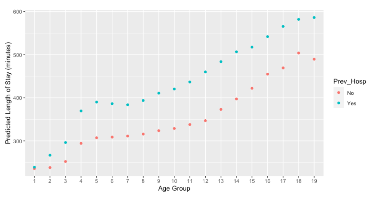
The PDP of the age group with the previous hospitalization status shows that patients with a history of previous hospitalization do have longer length of stays than those without, across all ages (the stay time increases with the age as well). Interestingly, in referral to the baseline characteristics table, the majority of people who come to the ED are those without previous hospitalization, but patients who do have a history of previous hospitalization tend to stay for longer. There is a noticeably large increase for those with previous hospitalization between the age groups of 3 (11 - 15) and 4 (16 - 20), suggesting that coming-of-age patients who have been previously hospitalized have a longer stay time; however, this gap is evidently smaller for patients without a previous hospitalization status. One rationale may be because both children and adults, although there is some great gap between the two, who have not been previously hospitalized are more likely to have less severe conditions that require less time to treat. There is also a large difference in the points of more senior patients: this indicates that there is some significant factor, most likely external, that causes previously hospitalized senior patients to have a longer stay time. One reason may be that having been previously hospitalized within three years indicates that the senior patient has already had a severe disease, which is more likely to relapse in older patients in intense severity and causing longer stay time; another conclusion could be that seniors who have not been previously hospitalized are likely to be healthier with less severe conditions. For either case, if the patient was aware of a condition that would require them to go to the ED, the stay time pre-transfer may be shorter.
Characteristics of Mispredicted Patients in the Regression Model
Due to the length of the table, it has been externally linked at https://docs.google.com/document/d/1mPWYJs6gXLMQZ4ta6VOjnhRhQ8DKY2HyBMRFIO9RJyE/edit?usp=sharing.
For the baseline characteristic to have little impact on the misprediction in the regression model, it should have a relatively consistent percentage across each of the mispredicted categories, such as biological assigned sex. However, for most variables, the misprediction time is diverse, ranging anywhere from generally decreasing percentage as the misprediction becomes greater (such as hospital type), generally increasing percentage as the misprediction becomes greater (such as rural patient postal districts), to sporadic (such as CTAS score). The most observable changes occurs in age group 1 (ages 1 - 5), where there is 12.2% mispredicted by less than 4 hours, but only 1.1% mispredicted by over 10 hours, category 5 for ICD-10 categories, where it increases from only 2.9% mispredicted by less than 4 hours to 29.1% mispredicted by over 10 hours, and large urban hospitals that increase from 43.2% mispredicted by less than 4 hours to 62.2% mispredicted by more than 10 hours. Additionally, for some sections of the table, such as biologically assigned sex and previous hospitalization status, more people are mispredicted for longer than 10 hours compared to the 4 - 10 hours categories. It may indicate that these characteristics have complex external factors that are difficult to completely predict with limited variables, likely causing a higher absolute residual value in the model.
Conclusion
Conclusion
Classification models have demonstrated considerable accuracy, especially the binary classification models. Regression models have the potential to make more accurate predictions when there are both a sufficient number of variables and data points. Due to the high complexity of the factors that contribute to a patient’s stay time in the ED, it is difficult to make specific and accurate predictions with the limited number and precision of variables. Comparing the classification and regression model performances, Random Forest classification may be more suitable for this datatset. All of the input variables are categorical, which makes it harder for the machine to accurately predict the length of stay to the exact minute. According to teh variable importance plot, the three most impactful variables were ICD 10 category, triage code, and age group. Categories 2 (neoplasms), 3 (diseases of the blood), 4 (endocrine, nutritional and metabolic diseases), and 5 (mental and behavioral disorders) generally had longer stay times; while categories 7 (diseases of the eye) and 8 (diseases of the ear) had the shortest length of stays comparatively. There may also be some difference in the stay time of underage and of age patients, where underage patients tend to have shorter length of stays regardless of the severity or previous hospitalization status; children’s hospitals may have more effective management and resource allocation, or children may be just given priority in some hospitals. Generally, the increase of age and an increase in severity of condition is also directly correlated with the inclination of predicted length of stay; patients who have been previously hospitalized within 3 years also have a higher chance of staying for longer than patients without.
Limitations
In the dataset, there was a rather limited number of variables compared to the large number of data. The input variables are categorical, making it difficult for the model to predict numerical values as the output. Potential variables that could be considered include the exact age instead of age group, laboratory and screening test requested, physical activity rate of the patient, BMI, smoking and alcohol consumption, medical history, economic status, and level of education. Moreover, the dataset consists of only 30% of ED visits in the years 2018 - 2020, which may limit the generalizability of the findings.
Future Work
Areas for improvement of the study would be to have a larger number of variables and more specific ones. For future analysis, the same dataset can be analyzed using other machine learning methods, where the results may be compared to Random Forest results to evaluate the efficacy of each machine learning model. Statistical analysis may also be employed to find correlations and the significance of independent variables.
Citations
Basic evaluation measures from the confusion matrix. (2015, June 3). Classifier Evaluation with Imbalanced Datasets; Classifier evaluation with imbalanced datasets. https://classeval.wordpress.com/introduction/basic-evaluation-measures/
Chugh, A. (2020, December 8). MAE, MSE, RMSE, Coefficient of Determination, Adjusted R Squared — Which Metric is Better? Medium. https://medium.com/analytics-vidhya/mae-mse-rmse-coefficient-of-determination-adjusted-r-squared-which-metric-is-better-cd0326a5697e
How is Variable Importance Calculated for a Random Forest? (2018, July 30). Displayr. https://www.displayr.com/how-is-variable-importance-calculated-for-a-random-forest/
IBM. (2023). What is Random Forest? | IBM. Www.ibm.com. https://www.ibm.com/topics/random-forest
Molnar, C. (n.d.). 5.1 Partial Dependence Plot (PDP) | Interpretable Machine Learning. In christophm.github.io. https://christophm.github.io/interpretable-ml-book/pdp.html
Out-of-Bag Error | Dremio. (n.d.). Www.dremio.com. Retrieved March 14, 2024, from https://www.dremio.com/wiki/out-of-bag-error/
Patient emergency department total length of stay (LOS) | HQCA Focus. (2024). Focus.hqca.ca. https://focus.hqca.ca/charts/total-length-of-patients-emergency-department-stay-los/
Random Forests · AFIT Data Science Lab R Programming Guide. (n.d.). Afit-R.github.io. https://afit-r.github.io/random_forests
Sruthi, E. R. (2021, June 17). Random Forest | Introduction to Random Forest Algorithm. Analytics Vidhya. https://www.analyticsvidhya.com/blog/2021/06/understanding-random-forest/
Taylor, C. (2019, January 27). What Are Residuals? ThoughtCo. https://www.thoughtco.com/what-are-residuals-3126253
THE CANADIAN TRIAGE AND ACUITY SCALE Combined Adult/Paediatric Educational Program PARTICIPANT’S MANUAL Triage Training Resources. (2007). http://ctas-phctas.ca/wp-content/uploads/2018/05/participant_manual_v2.5b_november_2013_0.pdf
What Is a Confusion Matrix in Machine Learning? (2022, August 18). Plat.AI. https://plat.ai/blog/confusion-matrix-in-machine-learning/
Wickramasinghe, S. (n.d.). Bias & Variance in Machine Learning: Concepts & Tutorials. BMC Blogs. https://www.bmc.com/blogs/bias-variance-machine-learning/
World Health Organization. (2019). ICD-10 Version:2019. Icd.who.int. https://icd.who.int/browse10/2019/en
Acknowledgement
Our deepest gratitude and appreciation to:
Dr. Jessalyn Holodinsky for mentoring us through this project,
Dr. Catherine Eastwood for helping us find a mentor at the department,
Dr. Bing Li for helping us find and use the dataset,
Ms. Jillian Vandenbrand for helping us schedule meetings with Dr. Jessalyn,
Our school teachers for the project registration,
and, lastly, our parents and friends for all of their support throughout this study.